The examples from Section 4.3 and Exercise 4.2.5 both embody the general idea of rate of change at a moment. They illustrated the idea that a moment $x_0$ is not an exact value.
By moment we shall mean a tiny interval containing values of an independent variable and which also contains $x_0$. When we spoke in Section 4.3 of the moment that a car’s motion was photographed, we had in mind the short period of time between when the shutter opened and when it closed.
"Moments" need not refer to moments in time. In Exercise 4.1.5, height was the independent variable. A moment while a function’s independent quantity varies is a tiny interval of values that includes a specific value of the independent quantity.
Moments vs. Exact Values
A variable can have exact values. When we say that h represents a height, we can envision that $h=6$ and we can say, "Let $h=6$".
But when we speak of the value of h varying, and we speak of "the moment when $h=6$ as the value of h varies", we are speaking of a tiny interval that includes $h=6$.
Remember: all motion, and hence all variation, is blurry.
Rate of Change at a Moment
We say that a function has a rate of change at the moment $x_0$ if, over
a suitably small interval of its independent variable containing $x_0$, the function’s value varies at essentially a constant rate with respect to its independent variable.
In this section we will examine examples of functions that have a rate of change at each moment while its independent variable varies. We will also examine functions that do not have a rate of change at any moment while its independent variable varies.
We will make the idea of rate of change at a moment more precise in a later section, and we will develop techniques for determining whether a function has a rate of change at a moment. Our goal, for the present, is that you form a productive image of what "rate of change at a moment" means.
Examples of Rate of Change at a Moment
Linear Functions
Linear functions are the simplest example of functions that have a rate of change at each moment while values of its independent variable vary. Indeed, they are so simple that it can be hard to see the idea of rate of change at a moment with them.
If f is linear over the real numbers, then it can be defined as $f(x) = m(x - a) + b$. This is the definition of a function whose graph passes through the point (a,b) with a constant rate of change m. For each value $x_0$ of x, f can be redefined as $f(x) = m(x - x_0) + f(x_0)$.
Therefore, over any interval containing $x_0$, f will have m as its constant rate of change with respect to x. Therefore, when f is linear, m is f’s rate of change at every moment as x varies.
Reflection 4.4.1. Restate the second sentence in the previous paragraph using the meaning of "moment". Do not use the word "moment".
Rate of Change at the Moment $x = x_0$ in $f(x) =
(x+1)^2 + 1$
Figure 4.4.1 shows two views of the graph of $y = f(x)$ where $f(x) = (x+1)^2 + 1$. At a normal scale, the graph of $y = f(x)$ appears non-linear, meaning it does not have a constant rate of change over any interval containing $x_0$. The graph on the right, however, is of $y = f(x)$ after zooming in on the graph repeatedly. The graph appears to be linear, suggesting that f has essentially a constant rate of change with respect to its independent variable over a suitably small interval containing $x_0$.
Figure 4.4.1. Graph of y = f(x) on the left at a normal scale; graph of y = f(x) zoomed in repeatedly around
the point $\left(x_0, f(x_0)\right)$, where $x_0=-1.36$. The graph on the left looks like there is no constant rate of change around $\left(x_0,f(x_0)\right)$. The graph on the right shows that f has a rate of change that is essentially constant over a small interval around $x_0$.
See this
video for the steps between starting with the graph on the left and ending with the zoomed graph on the right. (There is one small error in the video. Can you see it?)
Reflection 4.4.2. Use Figure 4.4.1 (right graph) to estimate the value of m, the rate of change of f at the moment $x = -1.36$.
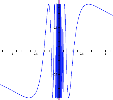
Rate of Change at the Moment that $x = 0.01701$ in $f(x) = \sin(\frac{1}{x})$
An earlier section discussed the behavior of $y = \sin(\frac{1}{x})$ for $x ≠ 0$. The wild gyrations in the graph as x approaches 0 from the right are because $\frac{1}{x}$ increases more and more rapidly as
x gets closer to 0, and therefore the argument to sine varies more and more rapidly through intervals of length 2π. The values of sine repeat themselves each time $\frac{1}{x}$ varies through an interval of length 2π. Therefore, the graph oscillates more and more rapidly as x approaches 0.
It might appear that for values of x near 0, $y = \sin(\frac{1}{x})$ cannot have a constant rate of change over even very small intervals. It seems to behave too crazily. The animation at this
link suggests otherwise. It suggests that over the interval $0.017099 ≤ x ≤ 0.017101$, $y = \sin(\frac{1}{x}$) has, essentially, a constant rate of change of 1204.94.
Figure 4.4.2. Graph of y =
sin($\frac{1}{x}$) over the interval $-1.25 < x < 1.15$.
See the animation at this
link for an explanation of why the rate of change of y with
respect to x at the moment that x=0.0171 is essentially 1204.94.
Our emphasize here is not so much that you can determine a function’s rate of change at specific moments. Rather, we want you to know what it means that a function has some number m as its rate of change at a moment $x=x_0$ of its independent variable. To repeat, it means that the function has essentially a constant rate of change m with respect to its independent variable over a suitably small interval surrounding $x_0$.
Put yet another way, a function f has a rate of change at the moment $x=x_0$ if there is a number m so that
$f(x_0+dx) \doteq f(x_0)+dy$, where $dy=m\,dx$, over a suitably small interval containing $x_0$.
Exercise Set 4.4
In Exercises 1-5 you are asked to experiment with finding an interval small enough around a given point so that the function appears to have a locally constant rate of change. The animation below illustrates working with Exercise 4.4.1.
Zoom in (shift-click-drag) enough times around the point ($x_0, g(x_0)$) so that you are convinced that this part of the graph displays a rate of change that is essentially constant over that interval.
Replace the value of $dx$ with an appropriate value to have GC calculate the constant rate of change over the interval you determined and to graph the linear function having that rate of change that passes through $(x_0, g(x_0))$. Set the value of $dx$ to make the arrows appear within your graph window.
Print your file. Write your answers to parts a-c below on the printout.
As you zoom in you eventually see two purple arrows. What do these arrows represent?
There is a command line in this file that calculates a value of m. Explain this calculation. Explain the value of m.
There is a command line in this file that graphs a linear function. Explain what this graph represents.
Zoom in (shift-click-drag) enough times around the point($x_0, g(x_0)$) so that you are convinced that this part of the graph displays a rate of change that is essentially constant over that interval.
Replace the value of $dx$ with an appropriate value to have GC calculate the constant rate of change over the interval you determined and to graph the linear function having that rate of change that passes through $(x_0, g(x_0))$. Set the value of $dx$ to make the arrows appear within your graph window.
Print your file. Write your answers to parts a-c below on the printout.
As you zoom in you eventually see two purple arrows. What do these arrows represent?
There is a command line in this file that calculates a value of m. Explain this calculation. Explain the value of m.
There is a command line in this file that graphs a linear function. Explain what this graph represents.
Zoom in (shift-click-drag) enough times around the point ($x_0, g(x_0)$) so that you are convinced that this part of the graph displays a rate of change that is essentially constant over that interval.
Replace the value of $dx$ with an appropriate value to have GC calculate the constant rate of change over the interval you determined and to graph the linear function having that rate of change that passes through $(x_0, g(x_0))$. Set the value of $dx$ to make the arrows appear within your graph window.
Print your file. Write your answers to parts a-c below on the printout.
As you zoom in you eventually see two purple arrows. What do these arrows represent?
There is a command line in this file that calculates a value of m. Explain this calculation. Explain the value of m.
There is a command line in this file that graphs a linear function. Explain what this graph represents.
What did you learn from doing Exercises 4.4.1 - 4.4.5?
In Exercise 4.3.1, no exact value of elapsed time was given as "the moment" that the camera’s shutter opened. How might we interpret the statement, "The moment when the camera’s shutter opened" so that it is consistent with the definition given in this section of rate of change at a moment?