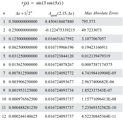
Figure 10.2.1. Table of values for $n$, $\Delta x=1/2^n$, $A_\mathrm{quad}(2,15,\Delta x)$, and $\left(\frac{15-2}{180}\right)176250(\Delta x)^4$
where $176250=\max\left|\dfrac{d^4}{dx^4}r_f(x)\right|$ for $2 \le x \le 15$.
| < Previous Section | Home | Next Section > |
In Section 10.1, we:.
Figure 10.2.1 shows a table of values like we saw in Section 10.1.
Figure 10.2.1. Table of values for $n$, $\Delta x=1/2^n$, $A_\mathrm{quad}(2,15,\Delta x)$, and $\left(\frac{15-2}{180}\right)176250(\Delta x)^4$
where $176250=\max\left|\dfrac{d^4}{dx^4}r_f(x)\right|$ for $2 \le x \le 15$.
Figure 10.2.1 gives information about how values of $A_\mathrm{quad}(2,15,\Delta x)$ behave as $\Delta x$ becomes smaller.
We can make other observations about rf and f in Figure 10.2.1.
The first observation is about maximum error of $A_\mathrm{quad}(a,x,\Delta x)$.
Put another way, if a rate of change function's 4th-order rate of change function is bounded over its domain, then the maximum absolute error of $A_\mathrm{quad}$ over that domain is proportional to $\left|x-a\right|$ for all values of x and a in the domain of $r_g$.
Reflection 10.2.1. Given $r_f(x)=\sin(3\cos(5x))$ What is the bound on maximum value of $\left|\int_5^{100} r_f(x) dx - A_\mathrm{quad}(5,100,0.02)\right|$?
What is the largest value of $\Delta x$ that will ensure $$\left|\int_0^{500b} r_g(t)dt-A_\mathrm{quad}(0,500b,\Delta x)\right|\le 0.00003$$ for all values of x, $0\le x \le 500b$?
The second observation is that our focus was largely on computing approximations to net accumulation. In approximating values of a net accumulation function f, however, we also approximated values of $r_f(x)$ for all values of x!
We approximated values of $r_f(x)$ with a polynomial of degree 0 (locally constant approximations of rf), degree 1 (locally linear approximations of rf), or degree 2 (locally quadratic approximations of rf).
Polynomial approximations of $r_f(x)$ for values of x gave us easily computable approximations to values of accumulation functions we could not compute directly.
However, there is a kink when we consider our quadratic approximation of an accumulation's rate of change function. We assumed we could compute any value of the rate of change function at any value of its domain.
Practically speaking, we were correct. GC computed values of sine, cosine, exponential and logarithmic functions for us. Someone figured a way to make computers capable to do these calculations and we used that capability. When $\sin(x)$ was our rate of change function, we had GC compute $\sin(\mathrm{left}((x))$, $\sin(\mathrm{mid}(x)$, and $\sin(\mathrm{right}(x))$ to generate our quadratic approximation of $\sin(x)$ over a $\Delta x$-interval.
In other words, we assumed we could calculate any value of the rate of change function for any value in its domain in our approximation of the rate of change function itself.
There was a time in human history when no one knew how to approximate values of non-algebraic functions like sine, cosine, exponential, and log. It is important we understand how this obstacle was overcome.
The third observation is about our general method of making stronger assumptions about the behavior of higher order rate of change functions for an accumulation function in order to make more accurate approximations of net accumulation with a given value of $\Delta x$.
In each of Observations 1-3, our approximation method was possible because we found algebraic simplifications of integrals over $\Delta x$-intervals that used values of $r_f$ as coefficients in our 0th-degree (constant), 1st-degree (linear), or 2nd-degree polynomial approximation of $r_f(x)$ over a $\Delta x$-interval.
But the algebra became more complicated as the degree of our polynomial approximations of rf increased.
Extending this general method to approximate variations in f by assuming $r_f^{(n)}(x)$ is essentially constant over $\Delta x$-intervals would require us to find a $(n-1)$-degree polynomial that passes through $(n-1)$ points on the graph of $y=r_f(x)$ in each $\Delta x$-interval.
It is possible, in principle, to find a polynomial of degree n passing through n distinct points in the plane. The method employs what is called polynomial interpolation, a topic beyond the scope of a calculus textbook. As an aside, the quadratic approximations to rate of change functions in Figures 10.1.14 and 10.1.15 were generated using polynomial interpolation.
Brook Taylor, building on earlier work by Barrow and Newton, took a different approach to approximating values of $r_f(x)$. He used polynomial functions to approximate a rate of change function, but his method for calculating coefficients of polynomial approximations to rf is more straighforward than polynomial interpolation.
The remainder of this section focuses on Taylor's method and its applications.
Suppose your programmable calculator has buttons for the variable x and for 0 - 9, +, -, *, $\div$, and $x^n$ for integers n. It also can graph $y=\cos(x)$ and other standard functions, but it cannot report values of these functions.
How might you calculate approximations of $\cos(x)$ for $-\pi\le x \le \pi$?
Let's start with a graph of $y=\cos(x),\,-\pi \le x \le \pi$.
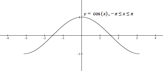
Figure 10.2.2. Graph of $y=\cos(x),\,-\pi \le x \le \pi$.
We are looking for a polynomial function of the form $p(x)=c_n x^n+c_{n-1} x^{n-1}+ \cdots +c_1x + c_0$ that gives a good approximation of $\cos(x)$ for every value of x, $-\pi\le x\le \pi$.
Focus on the graph around $x=0$. This part of the graph resembles $y=1-x^2$. Try it. (See Figure 10.2.3).
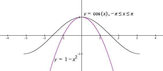
Figure 10.2.3. Graphs of $y=\cos(x),\,-\pi \le x \le \pi$ and $y=1-x^2$.
The graph of $y=1-x^2$ is close to $y=\cos(x)$ for values of x near 0, but $x^2$ becomes large too quickly for $\left| x \right|$ away from 0 and hence, as an approximation of $\cos(x)$, $1-x^2$ decreases too rapidly for $\left| x \right|$ away from 0.
Try $1-x^2/2$. The graph should decrease less rapidly (Figure 10.2.4).
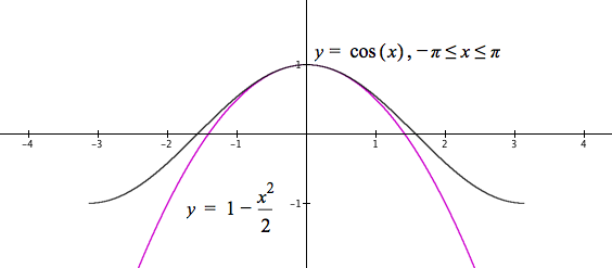
Figure 10.2.4. Graphs of $y=\cos(x),\,-\pi \le x \le \pi$ and $y=1-x^2/2$.
Figure 10.2.4 shows a close approximation of $y=1-x^2/2$ to $y=\cos(x)$ for $\left| x \right|\lt 1$, but the graph of $y=\cos(x)$ changes concavity around $\left| x \right|=\pi/2$ whereas $y=1-x^2/2$ does not.
We need to add another term that causes the graph of our polynomial approximation to begin turning up around $\left| x \right|=\pi/2$.
We cannot add an $x^3$ term. That would make the right side bend up but the left side bend down more than it does. The additional term must add a positive amount for both positive and negative values of x. So try adding $x^4/c$ where c is large enough to add little for small values of $\left| x \right|\approx 1$. Try adding $x^4/10$ (see Figure 10.2.5).
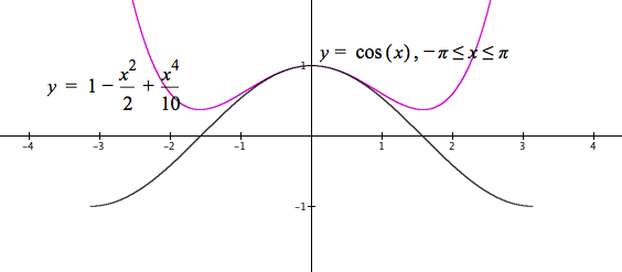
Figure 10.2.5. Graphs of $y=\cos(x),\,-\pi \le x \le \pi$ and $y=1-x^2/2+x^4/10$.
Values of $x^4/10$ are still too large away from 0. They add too much to $1-x^2/2$. We need to add a smaller multiple of $x^4$.
Some experimentation shows $x^4/28$ seems to work (see Figure 10.2.6.)
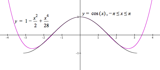
Figure 10.2.6. Graphs of $y=\cos(x),\,-\pi \le x \le \pi$ and $y=1-x^2/2+x^4/28$.
Reflection 10.2.4. Use the same style of graphical reasoning for building a polynomial approximation of $\cos(x)$ to build a polynomial approximation of $\sin(x),\, -\pi\le x \le \pi$.
One way to check our polynomial approximation of $\cos(x)$ is to draw on our knowledge of properties of $\cos(x)$, such as $\dfrac{d}{dx}\cos(x)=-\sin(x)$.
If $p(x)=1-\dfrac{x^2}{2}+\dfrac{x^4}{28}-\dfrac{x^6}{800}$ is our approximation of $\cos(x)$, then the graph of $$\begin{align} y&=\dfrac{d}{dx}p(x)\\[1ex]&=-x+\dfrac{4}{28}x^3-\dfrac{6}{800}x^5\end{align}$$ should resemble the graph of $y=-\sin(x)$, the derivative of $\cos(x)$, in a neighborhood of $x=0$. See Figure 10.2.7.
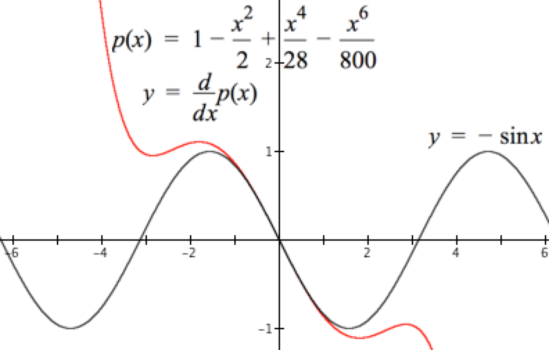
Figure 10.2.7. Graphs of $y=-\sin(x),\,-\pi \le x \le \pi$ and $y=\dfrac{d}{dx}p(x)$.
Figure 10.2.7 shows the graphs of $y=-\sin(x)$ and $y=-x+\frac{4}{28}x^3-\frac{6}{800}x^5$. The two do resemble each other in the neighborhood of $x=0$.
Our graphical approach to approximating $\cos(x)$ worked to some extent, but our unsystematic search for additional terms and coefficients does not guarantee a best approximation of rf.
A more systematic approach has its seeds in an observation we made about our approximation of $f(x)=\cos(x)$. It was that if $p(x)$ approximates $f(x)$, then the graph of $y=\dfrac{d}{dx}p(x)$ should approximate the graph of $y=-\sin(x)$ because $$\begin{align} \frac{d}{dx}f(x)&=\frac{d}{dx}\cos(x)\\[1ex] &=-\sin(x). \end{align}$$
Let $f(x)=\cos(x)$ be the function we wish to approximate and let a be a value in the domain of f.
Let $$p_n(x)=c_n(x-a)^n+c_{n-1}(x-a)^{n-1}+c_{n-2}(x-a)^{n-2}+\cdots + c_2(x-a)^2+c_1(x-a)+c_0$$ be the $n^{th}$-degree polynomial that approximates f for values of x near a. Our central question is, "What are the values of $c_n,\,c_{n-1},\,\cdots,c_2,\, c_1$, and $c_0$ that make $p_n$ satisfy the two conditions given above?"
$p_n(a)=0+0+\cdots +0+c_0$.
Let $c_0=f(a)$.
Then $p_n(a)=f(a)$. Condition #1 is satisfied when $c_0$ is defined as $c_0=f(a)$.
$\begin{align} r_{(p_n)}^{(1)}(x)&=\frac{d}{dx}p_n(x)\\[1ex] &=nc_n(x-a)^{n-1}+(n-1)c_{n-1}(x-a)^{n-2}+\cdots +3c_3(x-a)^2+2c_2(x-a) + c_1\\[1ex]\end{align}$.
So, $r_{(p_n)}^{(1)}(a)=c_1$.
Let $c_1=r_f(a)$.
Then $r_{(p_n)}^{(1)}(x)=r_f^{(1)}(x)$. The 1st-order rate of change function for $p_n$ and f agree for values of x near $x=a$ when $c_1$ and $c_0$ are defined as above. Condition #2 is satisfied for $k=1$.
$\begin{align} r_{(p_n)}^{(2)}(x)&=\frac{d}{dx}r_{(p_n)}^{(1)}(x))\\[1ex] &=n(n-1)c_n(x-a)^{n-2}+(n-1)(n-2)c_{n-1}(x-a)^{n-2}+\cdots + (3\cdot 2)(x-a) + 2c_2\\[1ex]\end{align}$.
So, $r_{(p_n)}^{(2)}(a)=2c_2$.
Let $c_2=\dfrac{r_f^{(2)}(a)}{2}$.
Then $r_{(p_n)}^{(2)}(x)=r_f^{(2)}(x)$. The 2nd-order rate of change function for $p_n$ and f agree for values of x near $x=a$ when $c_2$, $c_1$, and $c_0$ are defined as above. Condition #2 is satisfied for $k=2$.
$\begin{align} r_{(p_n)}^{(3)}(x)&=\frac{d}{dx}r_{(p_n)}^{(2)}(x))\\[1ex] &=n(n-1)(n-2)c_n(x-a)^{n-3}+(n-1)(n-2)(n-3)c_{n-1}(x-a)^{n-3}+\cdots +(4\cdot 3\cdot 2)(x-a) + (3\cdot 2) c_3\\[1ex]\end{align}$.
So, $r_{(p_n)}^{(3)}(a)=(3\cdot2)c_3$.
Let $c_3=\dfrac{r_f^{(3)}(a)}{3\cdot 2}$.
Then $r_{(p_n)}^{(3)}(x)=r_f^{(3)}(x)$. The 3rd-order rate of change function for $p_n$ and f agree for values of x near $x=a$ when $c_3$, $c_2$, $c_1$, and $c_0$ are defined as above. Condition #2 is satisfied for $k=3$.
$\begin{align} r_{(p_n)}^{(4)}(x)&=\frac{d}{dx}r_{(p_n)}^{(3)}(x))\\[1ex] &=n(n-1)(n-2)(n-3)c_n(x-a)^{n-4}+(n-1)(n-2)(n-3)(n-4)c_{n-1}(x-a)^{n-4}+\\ &\qquad \cdots +(5\cdot 4\cdot 3\cdot 2)(x-a) + (4\cdot 3\cdot 2)c_3\\[1ex]\end{align}$.
So, $r_{(p_n)}^{(4)}(a)=(4\cdot 3\cdot2)c_4$.
Let $c_4=\dfrac{r_f^{(4)}(a)}{4\cdot 3\cdot 2}$.
Then $r_{(p_n)}^{(4)}(x)=r_f^{(4)}(x)$. The 4th-order rate of change function for $p_n$ and f agree for values of x near $x=a$ when $c_4$, $c_3$, $c_2$, $c_1$, and $c_0$ are defined as above. Condition #2 is satisfied for $k=4$.
We can generalize this pattern: For a function f and values of x near a, $r_{(p_n)}^{(m)}$, the mth-order rate of change function for $p_n$, agrees with $r_f^{(m)}$, the mthorder rate of change function for f, when $$c_k=\dfrac{r_f^{(k)}(a)}{k(k-1)(k-2)\cdots 2\cdot 1}$$ for $k=0$ to $k=m$. Take note: $r_f^{(0)}(x)=f(x)$.
Using factorial notation, and recalling that $0!=1$, $$r_{(p_n)}^{(m)}(x)=r_f^{(m)}(x)\text{ when }c_k=\dfrac{r_f^{(k)}(a)}{k!}$$in the definiton of $p_n$. Fortunately for us, GC understands factorial notation.
In other words, the mth-order rate of change function for f agrees with the mth-order rate of change function for $p_n$ when the coefficient of $(x-a)^k$ is as stated above.
The final form of $p_n$ as a function whose values approximate $f(x)$ when x is near a is therefore $$\color{red}{\text{(Eq. 10.2.1)}}\qquad p_{n}(x)=f(a)+r_f^{(1)}(a)(x-a)+\frac{r_f^{(2)}(a)}{2!}(x-a)^2+\frac{r_f^{(3)}(a)}{3!}(x-a)^3+\cdots +\frac{r_f^{(n)}(a)}{n!}(x-a)^n$$
A polynomial in the form of Equation 10.2.1 is called a Taylor polynomial, after Brook Taylor.
We now return to the problem of approximating values of $\cos(x),\, -\pi\le x \le \pi$. We first think of approximating $\cos(x)$ with $a=0$. The value $a=0$ is conventient because $\cos(0)=1$ and $\sin(0)=0$.
To use a 10th-degree polynomial to approximate $\cos(x)$, we need $$\frac{d^k}{dx^k}\cos(x)$$ for $k=0$ to $k=10$, each evaluated at $a=0$, to compute $c_k$ for $k=0$ to $k=10$.
The table in Figure 10.2.8 gives all the information we need. The table also shows a clear pattern. By convention, $r_f^{(0)}(x)=f(x)$.

Figure 10.2.8. Rate of change functions for cos(x) of order $k\in\{0,1,2, ..., 10\}$.
The 10th-degree Taylor polynomial approximation for $f(x)=\cos(x)$ for $a=0$ and $-\pi\le x \le \pi$ is $$\begin{align} p_{10}(x)&=1+\frac{0x}{1!}-\frac{1x^2}{2!}+\frac{0x^3}{3!}+\frac{1x^4}{4!}+\frac{0x^5}{5!}-\frac{1x^6}{6!}+\frac{0x^7}{7!}+\frac{1x^8}{8!}+\frac{0x^9}{9!}-\frac{1x^{10}}{10!}\\[1ex] &=1-\frac{x^2}{2!}+\frac{x^4}{4!}-\frac{x^6}{6!}+\frac{x^8}{8!}-\frac{x^{10}}{10!}\end{align}$$
In Reflection 10.2.5 you determined that the relative error of $p_{10}(\pi)$ is approximately 0.0018, or 18/100 of 1%. You can compute $\cos(x),\, -\pi \le x \le \pi$ to a high degree of accuracy using just the 0 - 9, +, -, *, and $x^n$ keys on your calculator.
Figure 10.2.9 illustrates the improvement in $p_n$'s approximation of $\cos(x)$ as the value of n increases.
Figure 10.2.9. Graphs of $y=p_n(x)$ in relation to $y=\cos(x)$ as the value of n increases from 0 to 22.
First, let's generalize our notation to make easier use of GC. Instead of denoting a nth-order polynomial as $p_n(x)$, we will denote it as $p(x,n)$.
The definition of $p(x,10)$ as $$p(x,10)=1-\frac{x^2}{2!}+\frac{x^4}{4!}-\frac{x^6}{6!}+\frac{x^8}{8!}-\frac{x^{10}}{10!}$$ is cumberson to write and cumbersome to enter into GC. Indeed, the higher the order of a Taylor polynomial approximation, the more cumbersome to write its definition fully.
The use of summation notation to define a Taylor polynomial approximation to a rate of change function will be useful in the same way as using summation notation made it possible to write the general definition of an approximate accumulation function.
The hard part of using summation notation is to define the general term appropriately. Figure 10.2.9 contains the general term for the Taylor polynomial approximation to $\cos(x-a)$ with $a=0$. The general term is $$\frac{x^{2k}}{(2k)!}\qquad k=0,\,1,\,\dots,\,n$$
Figure 10.2.10 shows how to use summation notation in GC to define $p_n$.
Figure 10.2.10. Defining $p(x,n)$ in GC.
Notice two things about Figure 10.2.10
Reflection 10.2.6. Expand $p(x,4)$ into an explicit sum, where $p(x,n)=\sum\limits_{k=0}^n \dfrac{x^{2k}}{(2k)!}$. Notice that successive terms do not change sign.
Figure 10.2.11 shows how to make successive terms alternate sign. It uses the property that
So, $(-1)^k=1$ when k is even; $(-1)^k=-1$ when k is odd. Multiply the general term by $(-1)^k$.
Figure 10.2.11. Use $(-1)^k$ to make successive terms alternate signs.
Your graph of $y=p(x,10)$ in Reflection 10.2.5 showed the graph departing greatly from the graph of $y=\cos(x)$ for $\left| x \right|>\pi$. Figure 10.2.9 shows the graph of $y=p(x,n)$ eventually departs from the graph of $y=\cos(x)$ no matter the value of n.
How, then, can we use $p(x,10)$, or even $p(x,20)$, to approximate $\cos(x)$ for all values of x?
The function we define to approximate $\cos(x)$ for all values of x relies on two properties of the cosine function:
The cosine function is periodic with period $2\pi$. This is because an angle measure of $x-2\pi n$ is equivalent to an angle measure of x. It islike going back n full revolutions on a circle. You end where you begin.
For $x\ge 0$, the value of $\left\lfloor \dfrac{x}{2\pi}\right\rfloor$ gives the number of intervals of length $2\pi$ between 0 and x.
We can therefore reduce all positive values of x to an equivalent value between 0 and $2\pi$ by computing $x-2\pi\left\lfloor\dfrac{x}{2\pi}\right\rfloor$. Define the function $m_{2\pi}$ as $$m_{2\pi}(x)=x-2\pi\left\lfloor\frac{x}{2\pi}\right\rfloor.$$
The function $m_{2\pi}$ will reduce any non-negative value of x to an equivalent value between 0 and $2\pi$.
The value of $\cos\left(m_{2\pi}(x)-\pi\right)$ will be the same as the value of $-\cos(x)$.
p ctrl-L \cos\ $\rightarrow$ ctrl-9 x , n =
to get the partial statement "$p_{\cos}(x,n)=$".
We can therefore redefine $p_{\cos}$ as $$\begin{align} \color{red}{\text{(Eq. 10.2.2)}}\qquad p_{\cos}(x,n)&=-p\left(\left(m_{2\pi}(x)-\pi\right),n\right)\\[1ex] \text{where}\qquad p(x,n)&=\sum\limits_{k=0}^n (-1)^{k+1}\frac{x^{2k}}{2k!}\\[1ex] \text{and}\qquad m_{2\pi}(x)&=x-2\pi\left\lfloor\frac{x}{2\pi}\right\rfloor \end{align}$$
$p_{\cos}(x,n)$ as defined in Equation 10.1.2 will approximate the value of $\cos(x)$ for $x\ge 0$ by evaluating $p_{\cos}(x,n)$ at a value of $x$ between $-\pi$ and $\pi$.
The end result, as illustrated in the right side of Figure 10.2.12, is that approximations of $\cos(x)$ by $p_{\cos}(x,n)$ are as good for all values of x as for values of x in the interval $-\pi \le x \le \pi$. The left side of Figure 10.2.12 shows this is not the case for $p(x,n)$.
Figure 10.2.12. Behaviors of $y=p(x,n)$ and $p_{\cos}(x,n)$ as the value of n increases. There is always a "tail" in $y=p(x,n)$ that departs from $y=\cos(x)$, whereas the graph of $y=p_{\cos}(x,n)$ is indistinguishable from $y=\cos(x)$ at this scale for $n\gt 4$.
Reflection 10.2.8. Define p, and $p_{\cos}$ as given above. Compare the graphs of $y=p(x,10)$, $y=p_{\cos}(x,10$, and $y=\cos(x)$. (1) Type ctrl-L \cos\ to get $p_{\cos}$. (2) Scale your horizontal axis to see $-20\le x \le 20$. You might need to hide the graph of $y=\cos(x)$ to see the graph of $y=p_{\cos}(x,10)$.
Reflection 10.2.9. We stated the condition, "For $x\ge 0$" as a basis for defining $m_{2\pi}$. Yet, as your graphs in Reflection 10.2.6 show, $p(x)=-p_{10}\left(m_{2\pi}(x)-\pi\right)$ also works for negative values of x. Why?
Equation 10.2.1 uses powers of $(x-a)$. This is for two reasons:
Reflection 10.2.10. Let $a=1$ in the Taylor polynomial approximation to $\cos(x)$. What problem do you encounter regarding approximating values of $\cos(x)$ for values of x near $x=1$? Remember! The only buttons on your calculator are x, 0 - 9, +, -, $\div$, *, and $x^n$ for integers n.
Understanding Equation 10.2.1.
Applying Equation 10.2.1
Practice with summation notation
Connections
In Exercise Set 10.2.1 you determined a Taylor polynomial approximation for $e^x$ with $a=0$:
$$\begin{align} p_\text{exp}(x,n)&=1+x+\frac{x^2}{2}+\frac{x^3}{6}+\frac{x^4}{12}+\cdots+\frac{x^n}{n!}\\[1ex] &=\sum\limits_{k=0}^n \frac{x^k}{k!} \end{align}$$
Figure 10.2.13 shows the behavior of $y=p_\text{exp}(x,m)$ as the value of m increases from 0 to 20.
Figure 10.2.13. Approximation of $r_f(x)=e^x$ by $p_\text{exp} (x,m)=\sum\limits_{k=0}^m\dfrac{x^k}{k!}$.
Figure 10.2.13 illustrates an important consideration regarding Taylor polynomial approximations:
For some functions (e.g., $f(x)=e^x$), given two values $x_0$ and $x_1$, a higher-degree approximation is required to approximate the function at $x_1$ at the same level of accuracy as at $x_0$.
The table in Figure 10.2.14 illustrates the point just made, but illustrates it numerically. Before discussing the table's entries it will be worthwhile to remind yourself of scientific notation.
The table's first two columns give values of x and values of ex to 3 significant digits. The 3rd and 6th columns give values of $p_\text{exp}(x,25)$ and $p_\text{exp}(x,50)$, respectively, to 3 significant digits, where $p_\text{exp}(x,n)=\sum\limits_{k=0}^n\dfrac{x^k}{k!}$.
The 4th column gives the absolute error of $p_\text{exp}(x,25)$; the 7th column gives the absolute error of $p_\text{exp}(x,50)$.
The 5th column gives the relative error of $p_\text{exp}(x,25)$; the 8th column gives the relative error of $p_\text{exp}(x,50)$. The GC file used to generate this table is here.
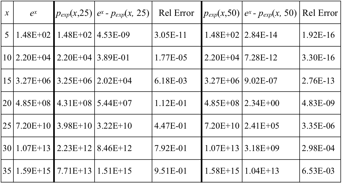
Figure 10.2.14. Table of values of ex and Taylor polynomial approximations of ex.
Comparing $p_\text{exp}(x,25)$ to ex
Reflection 10.2.11. Make comparisons of $p_\text{exp}(x,50)$ and ex similar to the comparisons of $p_\text{exp}(x,25)$ and ex.
Historically, Taylor polynomial approximations were a breakthrough for astronemers, natural philosophers (physicists), and mathematicians. They could approximate values of common non-algebraic functions using the first few terms of a Taylor polynomial.
Advances in numerical analysis brought methods superior to Taylor polynomials. These have been crystalized into standards set by the Institute of Electrical and Electronics Engineers (IEEE). The CORDIC method was a foundational advance for performing approximations on digital devices.
GC does not use Taylor polynomials. It uses IEEE routines for approximating values of non-algebraic functions. It will nevertheless be instructive for us to explore ways to improve Taylor polynomial approximations.
We saw earlier that we could improve approximations of $\cos(x)$ for large vaues of x by employing periodicity to our advantage. We defined $m_{2\pi}$ to transform any value of x to an equivalent value between 0 and $2\pi$ and used the fact that $\cos(x-\pi)=-\cos(x)$.
We then redefined $p_{\cos}$ as $$\begin{align}p_{\cos}(x,n)&=-p(m_{2\pi}(x)-\pi,n)\\[1ex] \text{where}\qquad p(x,n)&=\sum\limits_{k=0}^n (-1)^{k+1}\dfrac{x^{2k}}{(2k)!}\\[1ex] \text{and}\qquad m_{2\pi}(x)&=x-2\pi \left\lfloor \frac{x}{2\pi}\right\rfloor \end{align}$$.
We can use similar trickery to improve appoximations of $e^x$ and $\ln(x)$ for large values of x, but not by transforming the value of x. Rather, we will transform the value of a, the center of an approximation, to improve approximations of $e^x$ and $\ln(x)$ for values of x that standard Taylor polynomials approximate poorly.
Better approximations of ex
For $e^x$ we will leverage the fact that $\frac{d^k}{dx^k}e^x=e^x$ for $k=1,\, 2,\, \dots$ . So the kth term in any Taylor polynomial approximation of $e^x$ around $x=a$ will be $\dfrac{e^a}{k!}(x-a)^k.$
Figure 10.2.15 illustrates how the selection of a value of a affects the graph of $y=p_\text{exp}(x,n)$.
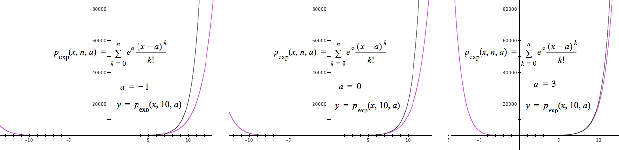
Figure 10.2.15
From the first bullet we can say $p(x,n,a)$ is most accurate for values of x near the value of a.
Our "trick" then is to use the integer nearest x from the left as our value of a, for every value of x. See Equation 10.2.3, below. $$ \color{red}{\text{(Eq. 10.2.3)}}\qquad p_\text{exp}(x,n)=\sum\limits_{k=0}^n \frac{e^{\lfloor x \rfloor}}{k!}(x-\lfloor x \rfloor)^k $$
Given that we must work with our restricted calculator, you might reasonably wonder about the legality of using $e^{\lfloor x \rfloor}$ in Equation 10.2.3. Think of it this way:
It is therefore legal to use $e^{\lfloor x \rfloor}$ in our definition of $p_\text{exp}$ in Equation 10.2.3.
Better approximations of ln(x)
We know $\frac{d}{dx}\ln(x)=x^{-1}$. The kth-order rate of change functions for $\ln(x)$ for $k=1,\,2,\,\dots,n$ are therefore
$x^{-1}$ (-1)x-2 (-2)(-1)x-3 (-3)(-2)(-1)x-4 ... $(-1)^{k+1}(k-1)!\, x^{-k}$
The Taylor polynomial for $\ln(x)$ centered at $x=a$ is therefore $$\begin{align} p_{\ln}(x,n)&=\ln(a)+\sum\limits_{k=1}^n (-1)^{k+1} \frac{a^{-k}}{k!} (k-1)!\,(x-a)^k\\[1ex] &=\ln(a)+\sum\limits_{k=1}^n (-1)^{k+1} \frac{a^{-k}}{k}(x-a)^k \end{align}$$
The accuracy of a Taylor polynomial approximation of $\ln(x)$ will therefore depend on judicious selection of the value of a.
First, we must pick a value of a for which we know $\ln(a)$. Since $\ln\left(e^c\right)=c$, powers of e work well.
Figure 10.2.16 shows the effect on Taylor approximations of $\ln(x)$ with $a=e^0,\,e^1,\,\dots,\,e^4$.
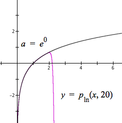
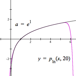
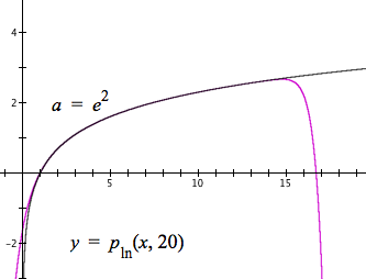
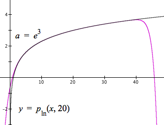
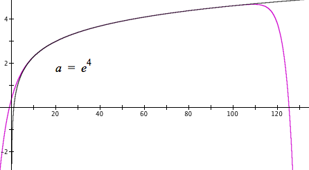
Figure 10.2.16. Taylor approximations of $\ln(x)$ using values of $e^k$ as values of a.
Figure 10.2.16 shows that as the value of x increases, we want to use a higher power of e as our value of a.
However, we need to devise a way to select powers of e algorithmically. The strategy used here will build on Figure 10.2.16. We start with a value of x and -4 as a value of m, then
We will define the function $a(x,m)$ to carry out steps 1-4 above.
The value of $a(x,m)$ will be, within defined range of possibilities, the least power of e that is greater than or equal to the value of x. We will use the value of $a(x,m)$ as the center (value of a) in the Taylor polynomial for each value of x. $$a(x,m)=\cases{ e^{-4} \qquad \text{if }x\le e^{-4}\\[1ex] e^{30} \qquad \text{if }x\ge e^{29}\\[1ex] e^m \qquad \text{if }e^m \ge x\\[1ex] a(x,m+1) }$$
For any value of x, $a(x,-4)$ will produce the least value of $e^m,\,-4\le m\le 30$, greater than or equal to x. The value -4 for m in $a(x,-4)$ is just to give m an initial value in the search for $e^m\ge x$. You msy use any integer as the intial value of m, and you msy use any integer for the upper value of $e^m$.
Our generalized Taylor polynomial for $\ln(x)$ is $$\color{red}{\text{(Eq. 10.2.4)}}\qquad p_{\ln}(x,n)=\ln(a(x,-4))+\sum\limits_{k=1}^n (-1)^{k+1}\frac{a(x,-4)^{-k}}{k}(x-a(x,-4))^k$$
You might wonder about using $\ln(a(x,-4))$ in the definition of $p_{\ln}$. It simply produces an integer value. How? The value of $a(x,-4)$ is a power of e, so $\ln(a(x,-4))$ is an integer (the exponent in the power of e).
If you are uncomfortable using $\ln(a(x,-4))$ in the definition of $p_{\ln}$, replace $\ln(a(x,-4))$ with $b(x,-4)$ where b is defined as
$$b(x,m)=\cases{ -4 \qquad \text{if }x\le e^{-4}\\[1ex] 30 \qquad \text{if }x\ge e^{29}\\[1ex] m \qquad \text{if }e^m \ge x\\[1ex] b(x,m+1) }$$
The value of $b(x,-4)$ is the exponent of e that $\ln(a(x,-4))$ produces.
You can increase the range of accuracy of $p_{\ln}$ for wider domains by changing the first two lines in the definitions of functions a and b. However, you will quickly exceed the capability of a 64-bit computer or calculator to make accurate calculations.
Reflection 10.2.15. Download and open this file. Use the q-slider. At what values of q is absolute error of $p_{\ln}(q,20)$ least? Greatest? Why?
A Taylor polynomial of degree n allows us to approximate any function f around $x=a$ for which $r_f^{(k)}(a)$ exists, $k\in\{0,1,\dots,n\}$.
Suppose $p_f(x,n)$ is a Taylor polynomial that approximates f around $x=a$. Then it seems reasonable to think that
In other words,
(More ...)
We will now address three issues that sat unacknowledged before our eyes.
(More ...)
We will see later that, in many cases, we can determine the degree of a Taylor polynomial approximation required to achieve a given accuracy level.
(More ...)
| < Previous Section | Home | Next Section > |