New Perspectives on Approximating Accumulation Functions from Rate of Change Functions
Assume essentially constant 1st-order rate of change of accumulation over small intervals
In Chapter 5 we employed the power of digital technologies to develop a method for approximating net accumulation from a reference point of a quantity when all we know is its exact rate of change function.
The method, in outline, was this:
Start with a known rate of change function rf, defined in closed form, whose values $r_f(x)$ give the exact rate of change of f at every moment x in the domain of f.
Assume a value $x=a$ from which net accumulation will be computed.
Define a function $r$ that approximates rf by assuming f varies at an essentially constant rate with respect to x as x varies by $dx$ over small intervals of length $\Delta x$. This assumption allows us to compute bits of accumulation $r(x)\,dx$ as $dx$ varies.
Define a function $A$ whose values $A(x)$ give the approximate net accumulation from $a$ to x
Define a function $A_f$, in open form, whose values $A_f(a,x)$ give the exact net accumulation in f from a to x.
Figure 10.1.1, repeated from Chapter 5, illustrates this process.
Figure 10.1.1. Visual summary of defining an exact net accumulation
function from an exact rate of change function.
Values of the function $A$, defined below, give the approximate accumulation in f from $a$ to x. (See Section
4.7 for a refresher on summation notation.)
Reflection 10.1.1. Where is dx
in the definition of A in Eq. 10.1.1?
The definition of $\mathrm{left}(x)$ assigns the value of the left end of a $\Delta x$-interval to each value of x in that interval (see the discussion of Figures
5.1.3 - 5.1.5).
The definition of $r$ makes $r(x)$ have the constant value $r_f(\mathrm{left}(x))$ for every value of x in any $\Delta x$-interval.
We could just as well define r using the value of rf at the midpoint of each $\Delta x$-interval (see Equation 10.1.2).
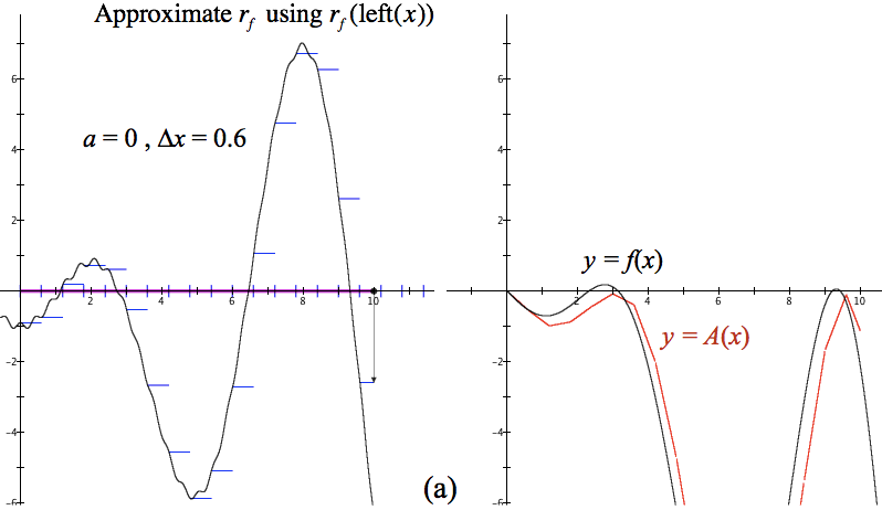
Examine Figures 10.1.2, 10.1.3, and 10.1.4. The definition of rf in each figure is $$r_f(x)=1.6\sin(x-2)+0.5-0.009(x-8)^2.$$ Each figure shows the graph of $y=r_f(x)$ and $y=r(x)$, with $a=-3$ and $\Delta x=0.6$, for one of the three methods of defining a constant function that approximates rf. The right panes show graphs of $y=A(x)$ according to each approximation of rf.
Figure 10.1.2. We approximate $r_f(x)$ over intervals $0\lt dx \le \Delta x$ with a function that is constant over each $\Delta x$-interval. The value of the constant function for each value of x in any $\Delta x$-interval is the value of rf at the left end of the interval.
Reflection 10.1.2.Where is $\Delta x$ in Figure 10.1.2? Where is dx in Figure 10.1.2? What influence does the value of $\Delta x$ have on the graph of y=A(x)?
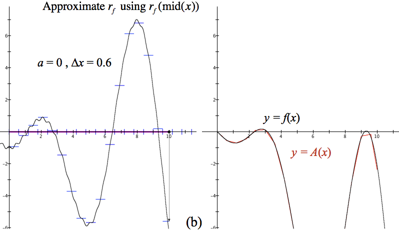
Figure 10.1.3. We approximate rf over intervals $0\lt dx \le \Delta x$ with a function that is constant over each $\Delta x$-interval. The value of the constant function for each value of x in any $\Delta x$-interval is the value of rf at the midpoint of the interval
Reflection 10.1.3. Where is $\Delta x$ in Figure 10.1.3? Where is dx in Figure 10.1.3? Why is the graph of y=r(x) in Figure 10.1.3 different from the graph of y=r(x) in Figure 10.1.2?
Reflection 10.1.4. Modify the definition of A in Eq. 10.1.1 using the definition of r in Eq. 10.1.2. Graph y=A(x) with $a=-3$ and $\Delta x=0.6$.
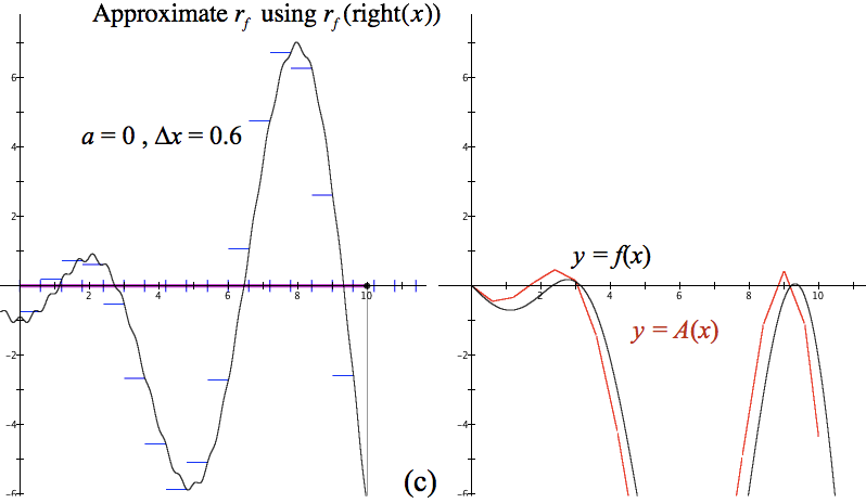
Figure 10.1.4. We approximate $r_f(x)$ over intervals $0\lt dx \le \Delta x$ with a function that is constant over each $\Delta x$-interval. The value of the constant function for each value of x in any $\Delta x$-interval is the value of rf at the right end of the interval.
Reflection 10.1.5. Modify the definition of r to use the value of rf at the right end of each $\Delta x$-interval. Modify the definition of A accordingly and graph y=A(x) in GC using $a=-3$ and $\Delta x=0.6$.
Reflection 10.1.6. Redefine rf as $r_f(x)=x \sin\left(2\pi \sqrt{x+3}\right)$. What would you need to change in Equations 10.1.1 or 10.1.2? Why? What would you need to change in your responses to Reflections 10.1.4 and 10.1.5? Why?
Approximation Error
Up until now we trusted we can make $\Delta x$ small enough so making it smaller makes no appreciable difference in the accuracy of the approximate accumulation function. We did not, however, investigate how good an approximation is for a particular value of $\Delta x$ or for particular values of x. We shall do that now.
Our explorations of how well an approximation method works will follow this pattern:
Start with an exact rate of change function having an exact accumulation function that can be defined in closed form.
Compare values of the approximate accumulation function with values of the exact accumulation function.
Create a method for determining upper and lower bounds for "error of approximation" (how far from exact our approximate accumulation function can be).
Apply our method for determining error of approximation of rate of change functions that have exact accumulation functions that cannot be defined in closed form.
There are several ways to judge how well an approximation method works for a particular rate of change function.
Inspection: Test the method on rate functions which have known accumulation functions in closed form. Compare graphs of approximate accumulation functions with the graph of the exact accumulation function
over intervals visible on the default screen
over larger intervals than are currently displayed
Closer inspection: Compare the difference (absolute error) or quotient (relative error) of the exact and approximate accumulation functions over small and large intervals
Numerically:
Examine the distance $\left|f(x)-A(x)\right|$ between the exact and approximate accumulation functions for values across their domains (absolute
error)
Examine the relative size of the absolute error and the exact value of the accumulation function $\left|\dfrac{ f(x)-A(x)}{f(x)}\right|, \, f(x)\neq 0$ (relative error)
Analytically: Create a formula that gives the maximum absolute or relative error of approximation for any value in the rate of change function's domain.
Absolute versus Relative Approximation Error
Let $F(x)$ be an exact net accumulation from a to x and let $A(x)$ be an approximate accumulation from a to x. Then absolute and relative approximation error are defined as:
Whether to focus on absolute or relative error is a matter of judgment.
If you are measuring the accumulated mass of microscopic particles, an absolute error of $3.7\times10^{-7}$ grams might seem very close to exact. If, however, a highly accurate measure is $5.1\times 10^{-8}$ grams, then your relative error is $$\frac{3.7\times10^{-7}}{5.1\times 10^{-8}}=7.255,$$ which means your approximation is off by a factor of 725.5%.
On the other hand, if you are measuring the distance to a star, an approximation having an absolute error of 2 billion kilometers might seem highly inaccurate. If, however, a highly accurate measure is 700.21 light-years, then your relative error is $$\frac{2\times10^9}{700.21\times 9.461\times 10^{12}}=0.0000302,$$or about 3/1000 of 1%.
Judging Approximation Error by Inspection
We know (using integration by parts) that $$\begin{align}
\int_0^x \left(t\sin(t)-1+0.1\cos(15t)\right)\,dt&=\left. -t+\sin(t)+\frac{2}{300}\sin(15t)-t\cos(t)\right|_{\,0}^{\,^x}\\[1ex]
&=-x+\sin(x)+\frac{2}{300}\sin(15x)-x\cos(x)
\end{align}$$
We can therefore compare our approximation methods against the exact accumulation function f defined as $$f(x)=-x+\sin(x)+\frac{2}{300}\sin(15x)-x\cos(x).$$
It might seem odd to approximate values of an accumulation function for which we can compute exact values or represent exact values in closed form. The purpose for approximating known values is not to approximate knownable values. Rather, the purpose is to judge how well approxmation methods work. Then we can use those methods with more or less confidence when approximating values of functions we cannot compute exactly.
Please download this
GC file to use in conjunction with the following discussion of Figures 10.1.5a through 10.1.5c.
Figure 10.1.5. Part (a) shows rf approximated by $r(\mathrm{left}(x))$ and the resulting graph of $y=A(x)$. Part (b) shows rf approximated by $r(\mathrm{mid}(x))$ and the resulting graph of $y=A(x)$. Part (c) shows rf approximated by $r(\mathrm{right}(x))$ and the resulting graph of $y=A(x)$.
Part (a) of Figure 10.1.5 shows, with this particular function rf, the definition of $r$ as $r(x)=r_f(\mathrm{left}(x))$ producing a constant rate of change that is a systematic under-approximation whenever rf increases over an interval and a systematic over-approximation when rf decreases over an interval.
Part (b) of Figure 10.1.5 shows the definition of $r$ as $r(x)=r_f(\mathrm{mid}(x))$ producing a constant rate of change that is an under-approximation for part of the interval and an over-approximation for the other when rf increases or decreases over the interval. The errors cancel each other to some extent.
Part (c) of Figure 10.1.5 shows the definition of $r$ as $r(x)=r_f(\mathrm{right}(x))$ producing a constant rate of change that systematically over-approximates rf when $r_f(x)$ increases over an interval and a systematic under-approximation when $r_f(x)$ decreases over an interval.
Reflection 10.1.7. In the GC
file for Figure 10.1.5, compare the absolute and relative error
over the interval defined by the slider named p by varying p's value.
Are your observations of these errors consistent with the graphs in
Figure 10.1.5?
Reflection 10.1.8. In the GC
file for Figure 10.1.5, reduce the value of $\Delta x$. Compare the absolute and relative error both graphically and by varying p's value. Are your observations of these errors still consistent with the graphs in Figure 10.1.5?
Reflection 10.1.9. In the GC
file for Figure 10.1.5, change the definition of rf to $r_f(x)=0.5\sqrt{x}e^{\cos(x)}$. Change the definition of f to $f(x)=\int_0^x 0.5\sqrt{t}e^{\cos(t)} dt$. Set $a=0$. Explore the absolute and relative error of the three methods of approximation.
Reflection 10.1.10. Sketch a graph of a function $r_g$ over a $\Delta x$-interval for which $r_g(\mathrm{left}(x))$ produces a better approximation of $r_g$ than does $r_g(\mathrm{mid}(x)))$. Explain what you mean by "better".
Reflection 10.1.11. Sketch a graph of a function $r_g$ over a $\Delta x$-interval for which $r_g(\mathrm{right}(x))$ produces a better approximation of $r_g$ than does $r_g(\mathrm{mid}(x)))$. Explain what you mean by "better".
Exercise Set 10.1.1
This GC file gives an alternative perspective on absolute and relative error as discussed in Figure 10.1.5.
Use the Method slider to compare absolute and relative errors of $A(x)$ for left, mid, and right methods of approximating rf over the displayed domain. Adjust the $\Delta x$-slider to see the effect of the value of $\Delta x$.
Explain what the blue graph shows.
Explain what the green graph shows.
For which method does $A(x)$ systematically give best approximations for $f(x)$?
Why does the value of relative error "spike" where it does regardless of the method you choose?
While the midpoint method generally produces more accurate approximate accumulation functions than the left or right method, the left or right method will sometimes work better than the midpoint method in particular cases.
Assume $\Delta x$=0.5 in (a) and (b).
Sketch the graph of a rate of change function for which the left method will produce the most accurate approximate accumulation function. Explain your answer.
Sketch the graph of a rate of change function for which the right method will produce the most accurate approximate accumulation function. Explain your answer.
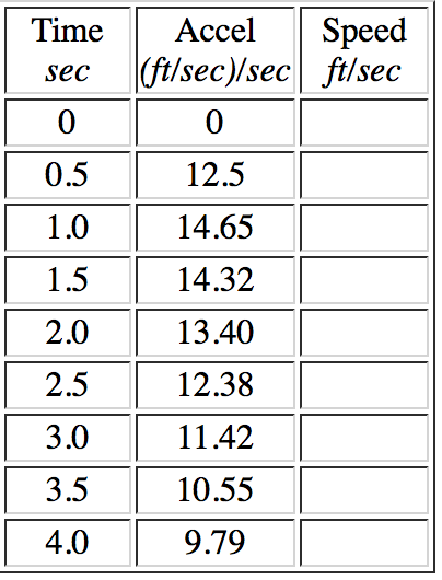
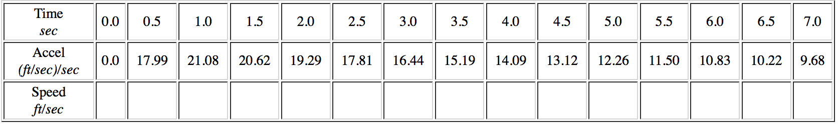
You can use a pendulum to measure an automobile's acceleration. It's angular displacement from vertical can be used to determine the auto's current forward or backward acceleration.
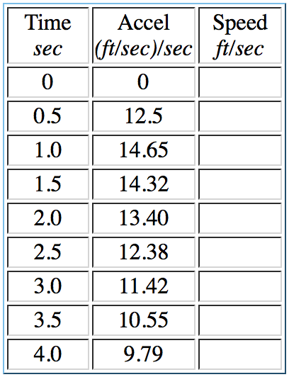
The table below provides a record of an automobile's acceleraton taken at intervals of 0.5 seconds. The car was traveling at 30 ft/sec at time $t=0$.
Save your results for this exercise. You will reuse them in Exercise Set 10.1.2.
What must you assume about the car's acceleration during each $\Delta x$-interval to use left or right method to approximate variations in its velocity when given only the data in this table? Why?
What must you assume about the car's acceleration during each $\Delta x$-interval to use mid method to approximate variations in its velocity when given only the data in this table? Why?
Use the left method to approximate the car's speed at the end of each 0.5-sec time interval.
Use the right method to approximate the car's speed at the end of each 0.5-sec time interval.
Use the mid-method to approximate the car's speed at the end of each 0.5-sec time interval. (Assume acceleration varies linearly over intervals.)
What are you assuming about the net accumulation function so acceleration varies linearly over intervals?
The car had a velocity at each moment after it began accelerating. Which of the three methods do you trust to give the most accurate approximation of the car's actual velocity over time? Why?
Other Approximation Methods
Review Chapter 7, Section 7.2 if you are unfamiliar with notations for higher-order rate of change functions.
The left-, mid-, and right- methods all derived from assuming that accumulation happens at an essentially constant rate of change over sufficiently small intervals.
Assuming accumulation happens at an essentially constant rate of change over sufficiently small intervals allowed us to approximate accumulation over an interval because we know how to compute accumulation from constant rate of change.
The methods we examine here follow the same logic. We will assume accumulation happens with an nth-order rate of change that is essentially constant over small intervals. This will imply that the accumulation's rate of change function is essentially a polynimial of degree $n-1$. And we know how to compute accumulation from polynomial rate of change functions!
Explore the above statement. Suppose f is an accumulation function.
If $r_f^{(2)}(x)$ is essentially constant over $\Delta x$-intervals, then $r_f(x)$ is essentially linear over $\Delta x$-intervals and $f(x)$ is essentially $Ax^2+Bx+C$ over those intervals.
If $r_f^{(3)}(x)$ is essentially constant over $\Delta x$-intervals, then $r_f(x)$ is essentially over $\Delta x$-intervals and $f(x)$ is essentially over those intervals.
If $r_f^{(4)}(x)$ is essentially constant over $\Delta x$-intervals, then $r_f(x)$ is essentially over $\Delta x$-intervals and $f(x)$ is essentially over those intervals.
Assume Essentially Constant 2nd-Order Rate of Change of Accumulation over Small Intervals
The three approximation methods (left-, mid-, right-) were all based on the idea of assuming an accumulation function has an essentially constant rate of change over sufficiently small $\Delta x$-intervals.
The differences among those approaches arose from our choice of where within a $\Delta x$-interval to take a value of rf as the constant rate of change that approximates the values of rf over that interval.
We approximated exact net accumulation by assuming accumulation happens at an essentially constant rate over each $\Delta x$-interval. We can also approximate exact net accumulation another way—assume accumulation happens with an essentially constant acceleration over each $\Delta x$-interval.
This would be the same as saying rf, the accumulation's rate of change function, varies essentially at a constant rate of change over each $\Delta x$-interval.
Figure 10.1.6 shows what it looks like to assume net accumulation varies with a constant acceleration over each $\Delta x$-interval.
Notice—by assuming net accumulation varies with an essentially constant acceleration over $\Delta x$-intervals, we thereby assume the accumulation's rate of change function rf varies esentially linearly (i.e., varies at a constant rate of change) over those intervals.
Figure 10.1.6. Approximate net accumulation function varies with an essentially
constant acceleration over $\Delta x$-intervals, which means that
approximate rate of change function varies essentially linearly (i.e., at a
constant rate of change) over each $\Delta x$-interval.
Our assumption that accumulation has an acceleration that is essentially constant over small $\Delta x$-intervals means we are also assuming rf is essentially linear (has a rate of change that is essentially constant) over each $\Delta x$-interval. This implies over any interval $[a,b]$, $r(x)$, rf's approximate rate of change function, has the form $r(x)=A(x-a)+B$ over $[a,b]$, where $A=\dfrac{r_f(b)-r_f(a)}{b-a}$ and $B=r_f(a)$.
Reflection 10.1.12. Why is $A=\dfrac{r_f(b)-r_f(a)}{b-a}$ and $B=r_f(a)$ when we say $r(x)=A(x-a)+B$ over the interval $[a,b]$?
The approximate accumulation function evaluated over an interval $a\le x\le b$ therefore has the value
Here is what we accomplished in Equation 10.1.3: Given an exact rate of change function rf, we can approximate net accumulation in f over a complete $\Delta x$-interval by computing $$\int_a^br_f(x)dx\approx\frac{r_f(a)+r_f(b)}{2}\Delta x$$ where $a$ and $b$ are the left and right ends, respectively, of the $\Delta x$-interval.
We can compute an approximate rate of change of accumulation over a partial $\Delta x$-interval from $\mathrm{left}(x)$ to x by computing $r_\text{cacc}(x)$ as $$r_\text{cacc}(x)=\frac{r_f(\mathrm{left}(x))+r_f(x)}{2}$$where "cacc" is short for "constant acceleration (of accumulation)", the assumption we made about how the approximate accumulation function varies. We can then compute the net accumulation in the current $\Delta x$-interval by $$r_\text{cacc}(x)\left(x-\mathrm{left}(x)\right)$$
In short, we can approximate exact net accumulation in f from $a$ to x by computing accumulation over the completed $\Delta x$-intervals included between $a$ and x, plus accumulation over the current, partial $\Delta x$-interval (see Equation 10.1.4).$$\color{red}{\text{(Eq. 10.1.4)}}\qquad A_\text{cacc}(x)=\left(\sum_{k=1}^\left\lfloor \frac {x-a}{\Delta x}\right\rfloor \left(\frac{r_f(a+(k-1)\Delta x)+r_f(a+k\Delta x)}{2}\right)\Delta x\right)+r_\text{cacc}(x)(x-\mathrm{left}(x))$$
Figure 10.1.9 shows linear approximation of rf and the resulting approximation of f by $A_\text{cacc}$ (assuming constant acceleration) with $\Delta x=0.6$. Figure 10.1.10 shows linear approximation of rf and the resulting approximation of f by $A_\text{cacc}$ (assuming constant acceleration) with $\Delta x=0.2$.
Figure 10.1.9. The graph of $y=A_\text{cacc}(x)$ with $\Delta
x$=0.6, where $A_\text{cacc}$ is the approximate net accumulation
function for f gotten by using $r_\mathrm{cacc}(x)$ as the
approximate rate of change of f with respect to x for every value
of x in a $\Delta x$-interval.
Reflection 10.1.13.
Explain why the graph of $y=A_\text{cacc}(x)$ must be
the graph of a quadratic function over every $\Delta x$-interval.
Figure 10.1.10. The graph of $y=A_\text{cacc}(x)$ with $\Delta x$=0.2, where $A_\text{cacc}$ is the approximate net accumulation function for f gotten by using $r_\mathrm{cacc}(x)$ as the approximate rate of change of f with respect to x over each $\Delta x$-interval.
Reflection 10.1.14.
Use GC to compare two methods of approximating exact accumulation, one using $A_\text{mid}(x)$ (assuming constant rate of change over intervals using mid-method) and one using using $A_\text{cacc}(x)$ (assuming accumulation with constant acceleration over intervals).
Use subscripts to differentiate between your two accumulation functions and your two approximate rate of change functions.
Refer to Equations 10.1.1, 10.1.2, and 10.1.4 for reminders.
Compare the accuracy of your new definitions graphically and numerically, using rf and f as shown below.$$\begin{align}r_f(x)&=\dfrac{e^{\cos x}}{1+e^{-x}}\\[1ex]f(x)&=\int_0^xr_f(t)dt\end{align}$$
Produce a table of your comparisons.
A More Convenient Notation For Approximate Net Accumulation
Until now we assigned the value of a, the reference value for net accumulation, outside the definition of A, the approximate net accumulation function.
However, the definition of exact net accumulation from exact rate of change,$$\int_a^x r_f(t)dt$$includes the values a and xwithin the definition. We therefor could define exact net accumulation in open form as $$A_f(a,x)=\int_a^x r_f(t)dt$$ to include the value of a explicitly.
We must also modify the definition of A, the approximate net accumulation function, to use a, x, and $\Delta x$ as arguments.
This requires us to modify the definitions of left( ), mid( ), right( ), r( ) to also use a, x, and $\Delta x$ as arguments.
We do this as in Equation 10.1.5. You may downlod a GC file with these functions here
Before the modifications introduced in Eq. 10.1.5 we had to enter, for example, $$\begin{align} a&=1.5\\[1ex] \Delta x&=0.20\\[1ex] y&=A_\mathrm{mid}(x) \end{align}.$$With the definitions in Eq. 10.1.5, we can get the same result by entering $$\begin{align} y=A_\mathrm{mid}(1.5,x,0.20)\end{align}$$
Notice: With net accumulation functions defined as in Eq. 10.1.5, we can compare approximations graphically by entering pairs of statements, like
$y=A_\mathrm{mid}(1,x,0.20)$ and $y=A_\mathrm{mid}(1,x,0.01)$
or
$y=A_\mathrm{cacc}(1,x,0.20)$ and $y=A_\mathrm{mid}(1,x,0.20)$
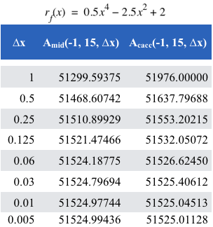
With the modified definitions in Equation 10.1.5 we can compare values of $A_\mathrm{mid}(a,x,\Delta x)$ and $A_\mathrm{cacc}(a,x,\Delta x)$ in a table that evaluates the approximations with different values of $\Delta x$, as shown below.
Quantifying Approximation Error
Remind yourself of the definitions of absolute and relative approximation errors. Given a reference value of $x=a$, an exact rate of change function rf for an exact net accumulation function F defined as $F(a,x)=\int_a^x r_f(t)dt$, and a value of $A(a,x,\Delta x)$ that approximates $F(a.x)$, then:
In your investigations, you probably noticed the midpoint method produced approximations to values of an exact accumulation function at least as accurate as the left, right, and constant acceleration methods, and often produced approximations noticeably better than the others.
The error in an approximation of an accumulation function's value is due not only to the method we use. It is also influenced by the size of $\Delta x$ in conjunction with the behavior of the accumulation function's rate of change function.
Figure 10.1.11 shows (on the left) graphs of $y=r_f(x)$, $\color{red}{y=r_\mathrm{mid}(a,x,\Delta x)}$, and $\color{blue}{y=r_\mathrm{cacc}(a,x,\Delta x)}$. It also shows (on the right) their respective accumulation functions as the value of $\Delta x$ changes from $\Delta x=1$ to $\Delta x=0.02$.
We recommend you watch the animation in Figure 10.1.11 several times, focusing first on the left pane, then on the right pane in relation to the left pane. Move your cursor away from the animation to make its scroll bar disappear.
Figure 10.1.11. Graphs of $y=r_f(x)$,
$y=r_{mid}(a,x,\Delta x)$, and $y=r_{cacc}(a,x,\Delta x)$ and their respective accumulation
functions as the value of $\Delta x$ changes from $\Delta x=1$ to $\Delta
x=0.02$.
Reflection 10.1.15.
Examine the left side of Figure 10.1.11 until you see:
$\Delta x$-intervals becoming smaller on the x-axis.
The graph of $y=r_\text{mid}(a,x,\Delta x)$, in $\color {red}{red}$, over each $\Delta x$-interval.
The graph of $y=r_\text{cacc}(a,x,\Delta x)$, in $\color {blue}{blue}$, over each $\Delta x$-interval.
Both graphs approach the graph of $y=r_f(x)$, in $\color {black}{black}$, over each $\Delta x$-interval.
Examine the right side of Figure 10.1.11 until you see:
The graph of $y=A_\text{mid}(a,x,\Delta x)$, in $\color {red}{red}$, over each $\Delta x$-interval.
The graph of $y=A_\text{cacc}(a,x,\Delta x)$, in $\color {blue}{blue}$, over each $\Delta x$-interval.
Both graphs approach the graph of $y=f(x)$, in $\color {black}{black}$, over each $\Delta x$-interval.
There is a lot to see in Figure 10.1.11. Drag the scroll bar to appropriate places in the animation as we focus on different aspects of what the animation illustrates.
Regarding approximations of $r_f(x)$:
Values of $r_\mathrm{mid}(x)$ and $r_\mathrm{cacc}(x)$, shown in the left pane, become closer to each other as the value of $\Delta x$ becomes smaller.
As the value of $\Delta x$ becomes smaller, both methods produce constant rates of change over $\Delta x$-intervals that become closer to the values of $r_f(x)$ over the same intervals.
For any given value of $\Delta x$, the faster $r_f(x)$ varies over that interval the farther apart are values of $r_\mathrm{mid}(x)$ and $r_\mathrm{cacc}(x)$. Using differential notation, the greater the value of $\dfrac{d^2}{dx^2}r_f(x)$ over an interval, the farther apart are values of $r_\mathrm{mid}(x)$ and $r_\mathrm{cacc}(x)$.
Regarding approximations of $f(x)$:
Values of $A_\mathrm{mid}(x)$ and $A_\mathrm{cacc}(x)$, shown in the right pane, become closer to each other as the value of $\Delta x$ becomes smaller.
As the value of $\Delta x$ becomes smaller, both methods produce approximate accumulations $\Delta x$-intervals that become closer to the values of $f(x)$ over the same intervals.
For any given value of $\Delta x$, the faster the rate of change of $r_f(x)$ varies with respect to x over an interval, the farther apart are values of $A_\mathrm{mid}(x)$ and $A_\mathrm{cacc}(x)$. Using differential notation, the greater the value of $\dfrac{d^2}{dx^2}r_f(x)$ over an interval, the farther apart are values of $A_\mathrm{mid}(x)$ and $A_\mathrm{cacc}(x)$.
As the value of $\Delta x$ becomes smaller, values of $A_\mathrm{mid}(x)$ become closer to values of $f(x)$ faster than do values of $A_\mathrm{cacc}(x)$.
Put another way, if we halve the value of $\Delta x$, the improvement in approximations of $f(x)$ over an interval by $A_\mathrm{mid}(x)$ tends to be greater than the improvement in the approximations of $f(x)$ by $A_\mathrm{cacc}(x)$.
Another way to look at these same observations is by building a table of values of $A_\mathrm{mid}(x)$ and $A_\mathrm{cacc}(x)$ for particular values of x and diminishing values of $\Delta x$.
The table in Figure 10.1.12 uses definitions of $A_\mathrm{mid}$ and $A_\mathrm{cacc}$ that are modified to accept the accumulation's reference value and the value of $\Delta x$ as arguments. We did this so we could hold the accumulation's reference value and end value constant while varying the value of $\Delta x$.
The GC file that produced Figure 10.1.12 is at this
link.
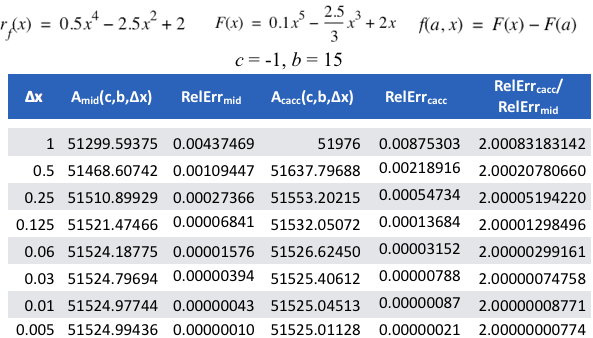
Figure 10.1.12. Values of $A_\mathrm{mid}(c.x,\Delta x)$ and
$A_\mathrm{cacc}(c,b,\Delta x)$ for
initial value of $c=-1$, $b=15$, and various values of $\Delta x$.
Inspect Figure 10.1.12 closely. Approximations of $f(-1,15)$ become better with smaller values of $\Delta x$. But there are two more things to see:
The relative error of either method improves steadily. Relative error, the magnitude of the absolute error of approximation in relation to the magnitude of $f(-1,15,\Delta x)$, becomes 1/4 as large each time the value of $\Delta x$ is made 1/2 as large.
This suggests relative error of either method is proportional to $(\Delta x)^2$.
Entries in the last column of Figure 10.1.12 show the relative size of the two relative errors. All entries are very close to 2, and get closer to 2 as $\Delta x$ becomes smaller. This means the relative error for $A_\mathrm{cacc}(-1,15,\Delta x)$ is always approximately twice as large as the relative error for $A_\mathrm{mid}(-1,15,\Delta x)$.
This is consistent with the bounds on actual error for $A_\mathrm{mid}$ and $A_\mathrm{cacc}$ given immediately above.
The bound for $A_\mathrm{mid}$ over an interval involves the quotient $\dfrac{x-a}{24}$ while the bound for $A_\mathrm{mid}$ involves the quotient $\dfrac{x-a}{12}$,
everything else is the same in both expressions.
In other words, the bound for maximum absolute error for $A_\mathrm{mid}$ is half as large as the bound for maximum absolute error for $A_\mathrm{cacc}$.
The actual upper bound for absolute error of the midpoint method is:$$\left|\int_a^xr_f(t)dt-A_\mathrm{mid}(a,x,\Delta x)\right|\le \left(\left(\frac{x-a}{24}\right) \left({\mathrm{max}\atop{a\le t \le x}} \left|\dfrac{d^2}{dt^2}r_f(t)\right|\right)\right)(\Delta x)^2.$$The actual upper bound for absolute error of the constant acceleration method is: $$\left|\int_a^xr_f(t)dt-A_\mathrm{cacc}(a,x,\Delta x)\right|\le \left(\left(\frac{x-a}{12}\right) \left({\mathrm{max}\atop{a\le t \le x}} \left|\dfrac{d^2}{dt^2}r_f(t)\right|\right)\right)(\Delta x)^2$$
You will see the reasoning for these bounds on absolute error later in Chapter 10.
In the meantime, notice:
the error bounds for $A_\mathrm{cacc}$ and $A_\mathrm{mid}$ are identical, except for the quotients $\dfrac{x-a}{12}$ and $\dfrac{x-a}{24}$.
The value of $\dfrac{x-a}{24}$ is half as large as the value of $\dfrac{x-a}{12}$.
This means bounds on approximations of $f(a,x)$ by $A_\mathrm{cacc}(a,x,∆x)$ are, in a general sense, twice as large (or half as accurate) as approximations of $f(a,x)$ by $A_\mathrm{mid}(a,x,\Delta x)$.
It is important to understand a bound on absolute error is not the same as actual absolute error. An error bound says the absolute approximate error cannot be any more than a certain value. It does not say what the actual error is.
Using GC to Calculate Error Bounds
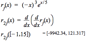
GC can provide approximations of a function's minimum and maximum values over an interval. Figure 10.1.13 shows how to use GC to find the min and max of $\dfrac{d^2}{dx^2}r_f(x)$ over the interval $[-1,15]$ where $r_f(x)=(-x)^3e^{x/5}$.
In GC, define rf and r2f as shown in Figure 10.1.13, typing ctrl-shift-D to get $\dfrac{d}{dx}$.
To type the third line of Figure 10.1.13, enter: r ctrl-L 2f (right arrow) ctrl-9 ctrl-[ -1 tab 15
Figure 10.1.13. Use GC to find min and max of the 2nd-order rate of change of rf over the interval $[-1,15]$.
Figure 10.1.13 shows the minimum and maximum values of $r_\text{2f}(x)$, the 2nd-order rate of change of rf over the interval $[-1,15]$ are approximately -9942.34 and -121.317, respectively, and hence $${\mathrm{max}\atop{-1\le x\le 15}} \left|\frac{d^2}{dx^2}r_f(x)\right|\approx 9942.34$$
According to error bounds on $A_\mathrm{mid}$, the maximum absolute error of $A_\mathrm{mid}(x)$ in comparison to $\int_{-1}^{15} r_f(t)\,dt$ over the interval $[-1,15]$ is $\dfrac{15+1}{24}\cdot 9942.34 (\Delta x)^2=6628.23(\Delta x)^2$. When $\Delta x=0.001$, the error bound is approximately $\pm 0.0795$.
Reflection 10.1.16. Use GC to compute $${\mathrm{max}\atop{-1\le t\le 15}} \left|\dfrac{d^2}{dt^2}r_f(t)\right|$$ for rf as defined in
Figure 10.1.12.
Use this value to compute the maximum relative error of $A_\mathrm{mid}(-1,15,0.25)$ as an approximation of $f(-1,15)$, where $f(a,x)$ is defined as in Figure 10.1.12.
Compare the maximum relative error you computed here with the appropriate entry in Figure 10.1.12. Are they consistent? Explain.
Reflection 10.1.17. The error bounds for both $A_\mathrm{mid}(x,\Delta x)$ and $A_\mathrm{cacc}(x,\Delta x)$ contain the term $$\left({\mathrm{max}\atop{a\le t \le x}} \left|\dfrac{d^2}{dt^2}r_f(t)\right|\right).$$Explain two things: (1) How this term means, "the largest value of the second derivative of $r_f(t)$ over the interval $a \le t \le x$", and (2) why the second derivative of rf might matter in determining maximum absolute error.
Reflection 10.1.18. Is the maximum relative error you computed for $A_\mathrm{mid}(-1,15,0.25)$ in Reflection 10.1.16 valid for all values of x from -1 to 15, or only for $x=15$? Explain.
Exercise Set 10.1.2
The table below is from Exercise 10.1.3. Approximate the car's velocity at the end of each time interval by computing $A_\text{cacc}(t)$ (see Equation 10.1.4) for each value of t in the table.
(Do not confuse the car's acceleration with assuming the car's velocity has an essentially constant acceleration.)
In GC,
Define the functions $r_G$, G, and g as $$\begin{align}r_G(x)&=e^{\sin x}\left((\cos x)^2-\sin x\right)\\[1ex] G(x)&=(\cos x)e^{\sin x}\\[1ex]g(a,x)&=G(x)-G(a).\end{align}$$Notice that G is an antiderivative of $r_G$.
Set GC to display 12 significant digits (in File/Document Settings).
Define $A_\text{mid}(a,x,\Delta x)$ in GC using rG as the exact rate of change function for G.
Define $r_{2G}$ as $\displaystyle{r_{2G}(x)=\frac{d}{dx}\left(\frac{d}{dx}r_G(x)\right)}$. Use a slider to estimate $\left(\displaystyle{{\mathrm{max}\atop{0\le t \le 5}} \left|r_{2G}(t)\right|}\right)$.
Use your estimate from (b) to estimate the maximum value of $\left| A_\text{mid}(0,x,0.1)-g(0,x)\right|$ over the interval $[0,5]$.
Use GC to compute the maximum value of $\left|A_\text{mid}(0,x,\Delta x)-g(0,x)\right|$ over the interval $[0,5]$ with values for $\Delta x$ of 1, 0.5, 0.25, and 0.125.
Are your estimates in Part (c) for the absolute error over the interval $[0,5]$ consistent the values you computed in Part (d)?
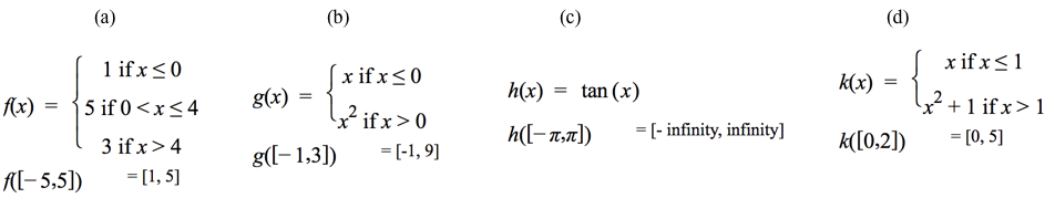
The range of a function over a domain D is the set of all values $f(x)$ such that $x\in D$.
We stated that the value of $f\left([a,b]\right)$ is a pair whose values give the minimum and maximum values of $f(x)$ over the interval $[a,b]$.
If f is continuous over $[a,b]$, then $f\left([a,b]\right)$ gives the lower and upper bounds of an interval constituting the range of f over $[a,b]$.
State for each of the following whether the function evaluated over the interval $[a,b]$ gives a pair that can also be taken as the lower and upper bounds of the function's range over $[a,b]$. If not, say why.
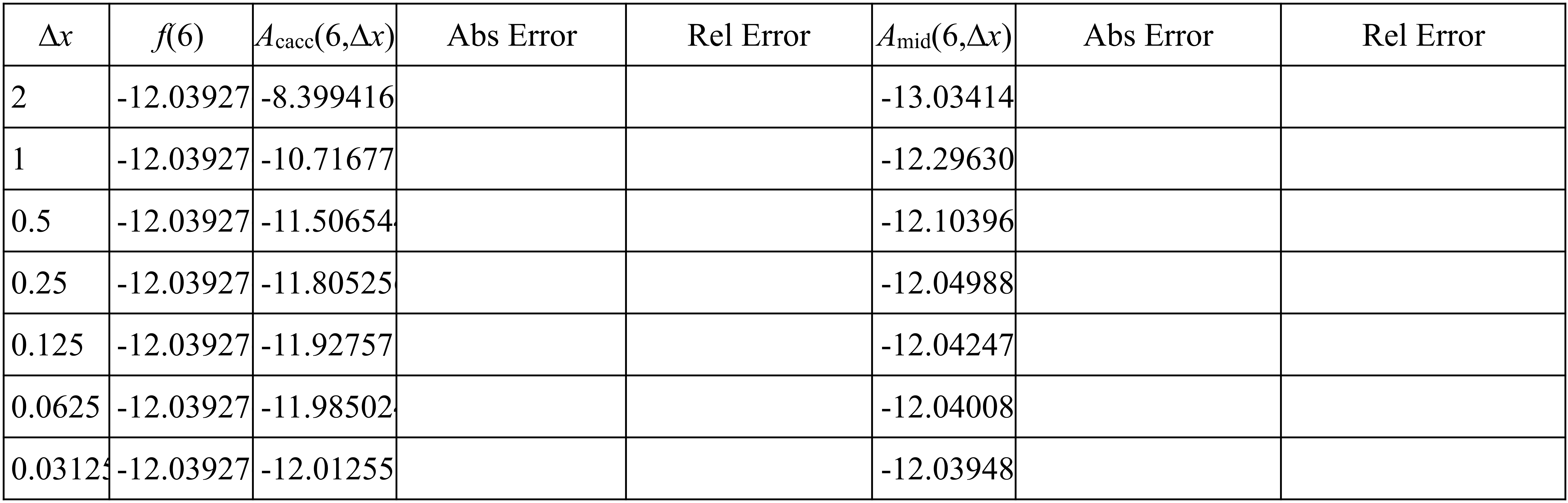
The table below has values of $A_\mathrm{left}(6,\Delta x)$ and $A_\mathrm{mid}(6,\Delta x)$ for a rate of change function rf defined over the interval $[0,6]$. The maximum value of $\left|\frac{d^2}{dx^2}r_f(x)\right|$ over $[0,6]$ is 24.
The values of $A_\mathrm{left}(6,\Delta x)$ and $A_\mathrm{mid}(6,\Delta x)$ are computed with various values of $\Delta x$. The table also has a column with the exact value of $f(6)$ to 8 significant digits.
Complete the table by computing maximum absolute and relative errors of each approximation. Suggestion: Define functions in GC to compute absolute and relative error.
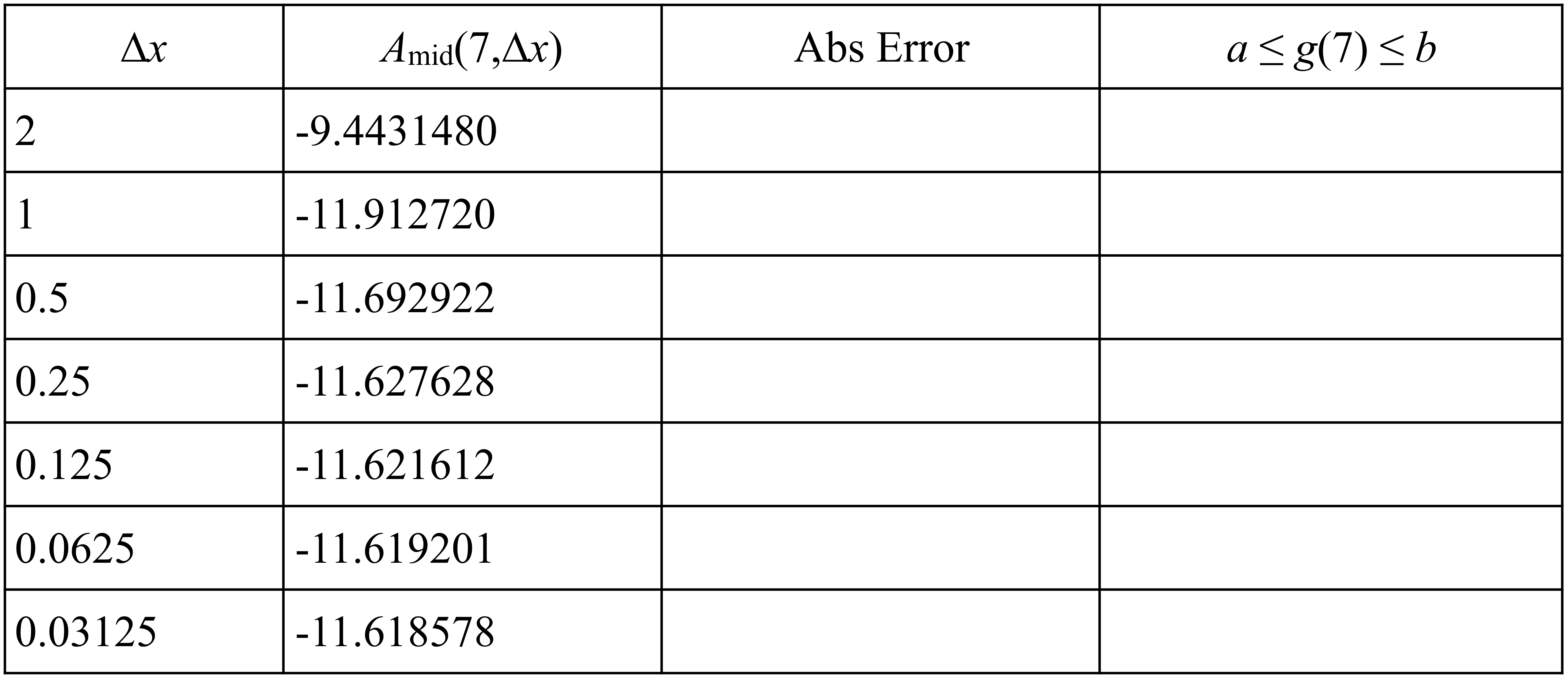
The table below has values of $A_\mathrm{mid}(7,\Delta x)$ as approximations of a net accumulation function g evaluated at $x=7$. The maximum value of $\left|\frac{d^2}{dx^2}r_g(x)\right|$ over $[0,7]$ is 25.
Complete the table by (1) computing maximum absolute approximation errors and (2) stating an interval $[a,b]$ containing $f(7)$ that your approximation error and estimate determines.
Assume Essentially Constant 3rd-order Rate of Change of Accumulation (constant jerk) Over Small Intervals
In the prior section we developed the method $A_\mathrm{cacc}$. The definitioin of $A_\mathrm{cacc}(a,x,\Delta x)$ used the rate of change half way between rf's values at each end of a $\Delta x$-interval as the constant rate of change of approximate accumulation as $dx$ varies through the interval.
We developed the constant acceleration method by assuming f, the exact accumulation function for rf, has an acceleration (2nd-order rate of change) that is essentially constant over $\Delta x$-intervals.
This assumption produced a method that was better than either the left( ) or right( ) methods, but not as good as using $r_f(\mathrm{mid}(x))$ as the constant rate of change of approximate accumulation over $\Delta x$-intervals.
A third method for approximating net accumulation from exact rate of change is to assume f, the exact accumulation function for rf, has a 3rd-order rate of change function (3rd derivative) that is essentially constant over each $\Delta x$-interval.
It would be reasonable to ask,
What good does it do to assume the exact accumulation function f has a 3rd-order rate of change function that is essentially constant over sufficiently small $\Delta x$-intervals?
Answer: Assuming f has an essentially constant 3rd-order rate of change function implies rf, the 1st-order rate of change function for f, is essentially quadratic over each $\Delta x$-interval. And we know
how to compute exact accumulation for a quadratic rate of change
function!
Reflection 10.1.19. Explain how
assuming an exact accumulation f has a 3rd-order rate of change
that is essentially constant over $\Delta x$-intervals implies its
1st-order rate of change function is essentially quadratic over the same
$\Delta x$-intervals.
Put another way, a quadratic approximation of rf over an interval is more sensitive to how rf varies over that interval than is a linear approximation of rf. A quadratic approximation of rf should therefore give us better approximations to the net change in accumulation over an interval than would linear approximations to rf over that interval.
Another advantage of using a quadratic function to approximate rf over an interval is we can approximate exact accumulation over complete $\Delta x$-intervals by computing the exact accumulation of the quadratic rate of change function that approximates rf over that $\Delta x$-interval.
Figure 10.1.14 illustrates the idea of approximating exact rate of change over an interval with a quadratic function over that same interval. The animations in Figure 10.1.14 use a sliding interval instead of a fixed interval to illustrate this approximation technique. This is only to show the technique works for any arbitrary interval. Move your cursor
away from an animation to make its scroll bar disappear.
(a) Quadratic approximation of rf over intervals of length 2.0.
(b) Quadratic approximation of rf over intervals of length 1.0.
(c) Quadratic approximation of rf over intervals of length 0.5.
Figure10.1.14. Three approximations to an exact rate of change
function by a quadratic function over an interval of length $\Delta
x$, with $\Delta x=2.0$, $\Delta x=1.0$, and $\Delta x=0.5$. The
intervals slide along the x-axis to illustrate quadratic approximation
over any interval.
(a) Left. Graph of $\color{red}{y=r_\mathrm{quad}(x)}$,
the quadratic approximation of $y=r_f(x)$ over intervals of length $\Delta x=1.0$. Heavy gray lines show left and right ends of successive $\Delta x$-intervals. Light gray lines show middles of $\Delta x$-intervals. Graph of $\color{red}{y=r_\mathrm{quad}(x)}$ passes through graph of $y=r_f(x)$ at left end, middle, and right end of each $\Delta x$-interval. Right. The
graph, $\color{green}{\text{in green}}$, of the exact
accumulation function from rf along with the graph of $\color{red}{A_\mathrm{quad}}$, the approximate accumulation function.
(b) Left. Graph
of $\color{red}{y=r_\mathrm{quad}(x)}$, the quadratic approximation of $y=r_f(x)$ over intervals of length $\Delta x=0.4$. Heavy gray lines show left and right ends of successive $\Delta x$-intervals. Light gray lines show middles of $\Delta x$-intervals. Graph of $\color{red}{y=r_\mathrm{quad}(x)}$ passes through graph of $y=r_f(x)$ at left end, middle, and right end of each $\Delta x$-interval. Right. The
graph, $\color{green}{\text{in green}}$, of the exact
accumulation function from rf along with the graph of $\color{red}{A_\mathrm{quad}}$, the approximate accumulation function.
Figure 10.1.15. (a) Quadratic approximation of rf with $\Delta x=1.0$. (b) Quadratic approximation of rf with $\Delta x=0.4$.
Approximate Accumulation from Quadratic Approximation of Exact Rate of Change
One thing remained common among the methods for approximating the exact accumulation function f from its exact rate of change function rf. We approximated rf with a function for which we knew how to compute exact accumulation over an interval from rate of change over that interval.
Our first three methods (left, mid, and right) assumed a constant rate of change over $\Delta x$-intervals, which made it easy to calculate approximate accumulation over every $\Delta x$-interval.
The constant acceleration method (linear approximation of rf) relied on the fact we can represent the integral of a linear function over an interval in closed form.
The situation with quadratic approximations to rf over $\Delta x$-intervals is like the constant acceleration method. We will calculate approximate accumulation over an interval from an approximate rate of change function that is quadratic over that interval.
Let rf be the exact rate of change function for an exact accumulation function f. Let $[a,b]$ be any interval in the domain of rf. The quadratic approximation of rf over this interval must be such that $r(a)=r_f(a)$, $r\left(\frac{a+b}{2}\right)=r_f\left(\frac{a+b}{2}\right)$, and $r(b)=r_f(b)$. In other words, the graph of the approximate rate function $r$ must pass through the graph of rf at the left, middle, and end values of $[a,b]$. Then,
However, we seem to have a stumbling block: We do not know the values of A, B, and C. But we do know three points the quadratic must pass through. It turns out we can use this information to produce a way to compute the value of $\int_a^b\left(Ax^2+Bx+c\right)dx$ without needing the values of A, B, and C.
Suppose rf is an exact rate of change function for f defined over an interval $[a.b]$. Suppose further $r$ is a quadratic function that agrees with rf at the left end, middle, and right end of $[a,b]$. This means that $r(x)=Ax^2+Bx+C$ such that
$$\begin{align}
\int_a^b r(x)dx&=\int_a^b\left(Ax^2+Bx+c\right)dx\\[1ex]
&=A\int_a^b x^2dx+ B\int_a^b x dx+C\int_a^b 1 dx\\[1ex]
&=A\frac{b^3-a^3}{3}+B\frac{b^2-a^2}{2}+C(b-a)\\[1ex]
&=A\frac{(b-a)(a^2+ab+b^2)}{3}+B\frac{(b-a)(b+a)}{2}+C(b-a)\\[1ex]
&=(b-a)\left(A\frac{a^2+ab+b^2}{3}+B(b+a)/2+C\right)\\[1ex]
&=\text{(... a bunch more algebra ...)}\\[1ex]
&=\frac{b-a}{3}\left(\frac{Aa^2+Ba+C}{2}+2\left(A\cdot\left(\frac{b+a}{2}\right)^2+B\cdot\left(\frac{b+a}{2}\right)+C\right)+
\frac{Ab^2+Bb+C}{2}\right)\\[1ex]
&=\frac{b-a}{3}\left( \frac{r(a)}{2}+2r\left( (b+a)/2\right)+\frac{r(b)}{2}\right)\\[1ex]
&=\frac{b-a}{3}\left( \frac{r_f(a)}{2}+2r_f((b+a)/2)+\frac{r_f(b)}{2}\right)\\[1ex]
\int_a^b r(x)dx&=\frac{b-a}{3}\left( \frac{r_f(a)}{2}+2r_f((b+a)/2)+\frac{r_f(b)}{2}\right)\end{align}$$
That is, we end up evaluating $\displaystyle{\int_a^br(x)dx}$ without having to know the coefficients A, B, and C in $r(x)=Ax^2+Bx+C$. All we need are the values of $r_f(x)$ at the interval's left end, midpoint, and right end.
We may now define a function $s$ that uses a quadratic approximation of rf to approximate the exact accumulation in f over an interval $[c,d]$:
and use the definition of s to approximate the net accumulation over an interval $[a,x]$ that contains $\left\lfloor\frac{x-a}{\Delta x}\right\rfloor$ complete intervals of length $\Delta x$.
The definitions of left, $s$, and $A_\mathrm{quad}$ given in Equation 10.1.6, entered into GC, were used to produce the animations in Figure 10.1.15.
Error Bound on Quadratic Approximation of Accumulation Functions
The error bound on the quadratic approximation method is much tighter than for the mid-point method, which you probably inferred from the animations in Figure 10.1.15. The error bound for the quadratic method is:
Compare the quadratic error bound with the error bound for the midpoint method:
$$\color{red}{\text{Mid Error Bound}}\qquad \left|\int_a^xr_f(t)dt-A_\mathrm{mid}(a,x,\Delta x)\right|\le \left(\left(\frac{x-a}{24}\right) \left({\mathrm{max}\atop{a\le t \le x}} \left|\dfrac{d^2}{dt^2}r_f(t)\right|\right)\right)(\Delta x)^2$$ Since the values of $$\dfrac{\displaystyle{{\mathrm{max}\atop{a\le t \le x}}} \left|\dfrac{d^2}{dt^2}r_f(t)\right|}{24}$$
and
$$\dfrac{\displaystyle{{\mathrm{max}\atop{a\le t \le x}}} \left|\dfrac{d^4}{dt^4}r_f(t)\right|}{180}$$
are constant for any value of x in $[a,b]$, the comparison in accuracy of the midpoint and quadratic methods depends essentially on values of $\Delta x^2$ and $\Delta x^4$.
Notice:
When $\Delta x=0.1$, $\Delta x^2=0.01$ and $\Delta x^4=0.0001$.
When $\Delta x=0.01$, $\Delta x^2=0.0001$ and $\Delta x^4=0.00000001$.
When $\Delta x=10^{-3}$, $\Delta x^2=10^{-6}$ and $\Delta x^4=10^{-12}$.
When $\Delta x=10^{-n}$, $\Delta x^2=10^{-2n}$ and $\Delta x^4=10^{-4n}$
The error bound for the quadratic method becomes smaller at a much faster rate than the error bound for the midpoint method as $\Delta x$ decreases in value.
This means, in principle, approximations using the quadratic method for small values of $\Delta x$ will be far more accurate than approximations using the midpoint method.
Use GC to Compute Maximum Absolute Error for $A_\mathrm{quad}(a,x,\Delta x)$
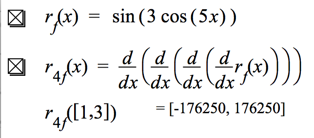
As with $A_\mathrm{mid}$, we can use GC to compute bounds on absolute approximation error for $A_\mathrm{quad}$ over an interval. Figure 10.1.16 shows how to do this with $r_f(x)=\sin(3\cos(5x))$.
Define r4f as shown in Figure 10.1.16.
Type ctrl-shift-D to get $\dfrac{d}{dx}$.
To type the third line of Figure 10.1.16, enter: r ctrl-L 4f (right arrow) ctrl-9 ctrl-[ 1 tab 3
Figure 10.1.16. Use GC to find min and max of the 4th-degree rate of change of rf over the interval $[1,3]$.
Figure 10.1.16 shows the minimum and maximum values of $r_\text{4f}(x)$ over the interval $[1,3]$ are -176250 and 176250, respectively.
The maximum absolute value of $r_\text{4f}(x)$ over the interval $[1,3]$ is therefore 176250, and hence $${\mathrm{max}\atop{1\le x\le 3}} \left|\frac{d^4}{dx^4}r_f(x)\right|\approx 176250$$
Reflection 10.1.20. Use GC to compute lower and upper bounds for the value of$$\int_0^2 e^{\cos (x-1)}\,dx$$when approximating it with $A_\mathrm{quad}(0,2,\Delta x)$. Use 0.5, 0.1, and 0.01 as values of $\Delta x$.
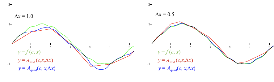
Figure 10.1.17 shows comparisons between $A_\mathrm{mid}$ and $A_\mathrm{quad}$, with $\Delta x=1.0$ on the left and $\Delta x=0.5$ on the right. It illustrates $A_\mathrm{quad}$ converges to the exact accumulation function faster than does $A_\mathrm{mid}$.
Figure 10.1.17. Comparisons of approximate
accumulation functions generated by the midpoint and quadratic approximations to rf.
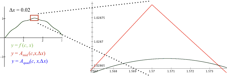
Figure 10.1.18 shows both approximation methods appearing to produce approximate accumulation functions that coincide with the exact accumulation function.
Figure 10.1.18. Comparing the midpoint and quadratic approximation
methods over the interval $[1.567,1.574]$. The graph of the quadratic
approximation function is indistinguishable from the graph of the exact
accumulation function while the graph of the midpoint approximation
function departs considerably in comparison.
However, an enlargment of one small section of the graph shows the approximate accumulation function given by the midpoint method deviates by a relatively large amount from exact accumulation in comparison to the quadratic approximation method.
Even at the zoom level of Figure 10.1.18 the quadratic approximate accumulation function is indistinguishable from the exact accumulation function.
Exercise Set 10.1.3
The table shows a car's acceleration recorded at half-second intervals. Approximate the car's velocity at the end of appropriate time intervals by computing values of $A_\text{quad}(t).$ (See Equation 10.1.6).
Remember $A_\text{quad}$ requires 3 values of rf !.
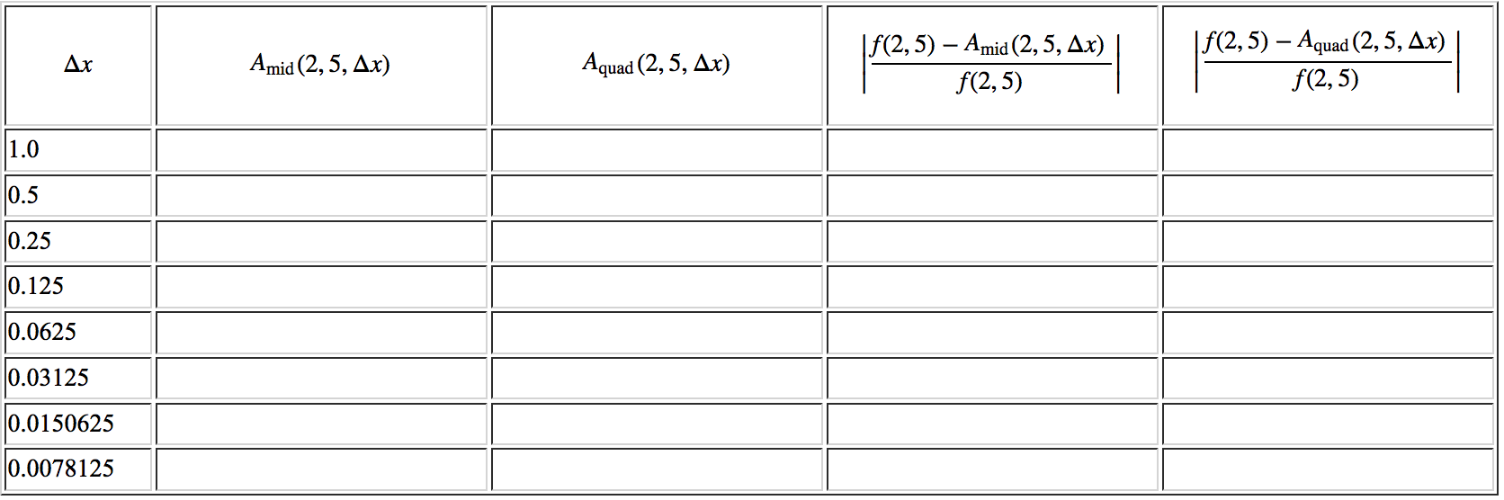
Let rf be defined as $r_f(x)=\cos(x)+0.3\sin(10x)$.
Define rf, $A_\mathrm{mid}$ and $A_\mathrm{quad}$ and all necessary auxiliary functions in GC.
Set GC to display 12 significant digits (File/Document Settings).
Use GC to fill in the following table. Check your work by clicking here to see the first row.
Notice each successive value of $\Delta x$ is half the preceding value. What does halving a value of $\Delta x$ do the respective values of $A_\mathrm{mid}(2,5,\Delta x)$ and $A_\mathrm{quad}(2,5,\Delta x)$?
The function rg defined as $r_g(x)=\cos(3x)e^{\cos x}$ does not have a closed-form antiderivative so we cannot check the accuracty of $A_\mathrm{quad}(a,x,\Delta x)$ against exact values of g.
Use GC to compute maximum value of $\left|A_\mathrm{quad}(0,3,0.01)-\int_0^3 r_g(t)\,dt\right|$. Use this computation to give lower and upper bounds for $\int_0^3 \cos(3t)e^{\cos t}dt$.
Convergence
Until now we compared values of approximate accumulation functions $A(x)$ for an exact accumulation function f that can be defined in closed form. This allowed us to compare our approximations at specific values of x with values of $f(x)$ we could compute directly from $f's$ closed form definition. We then inspected the accuracy of various approximation methods by comparing them to values of an exact accumulation function. We determined the quadratic approximation method is better by far than any of the other methods we inspected.
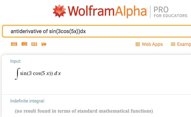
As we stated in Section 10.0, the vast majority of accumulation functions you will meet in applied settings cannot be represented in closed form. A seemingly simple case is $r_f(x)=\sin(3\cos(5x))$. Here is what Wolfram Alpha Pro reports when asked for an antiderivative of $\sin(3\cos(5x))$.
Figure 10.1.19. The result of Wolfram Alpha Pro's attempt to determine
an antiderivative of $\sin(3\cos(5x))$. It could not determine one.
In the case of $r_f(x)=\sin(3\cos(5x))$, we cannot calculate exact accumulation values against which to compare our approximate accumulation values.
With what values, then, do we compare our approximations? The answer is, "with each other".
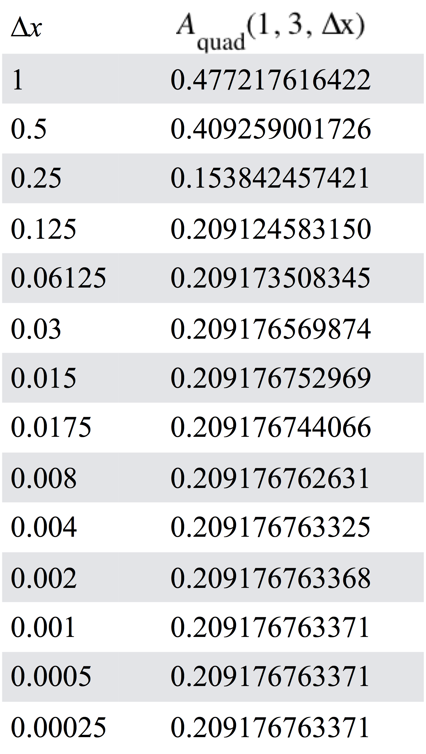
Figure 10.1.20 gives two columns of numbers. The first column contains values of $\Delta x$. The second column contains values (to 12 significant digits) of $A_\mathrm{quad}(1, 3, \Delta x)$, where $A_\mathrm{quad}(1,3,\Delta x)$ is defined in terms of $r_f(x)=\sin(3\cos(5x)$.
Figure 10.1.20. Table of values for $A_\mathrm{quad}(1,3,\Delta x)$
with $r_f(x)=\sin(3\cos(5x))$ and varying values of $\Delta x$.
Reading Figure 10.1.20 from the top, we see values of $A_\mathrm{quad}(1,3,\Delta x)$ agree with each other in more decimal places as values of $\Delta x$ become smaller. This is true until $\Delta x$ has a value of 0.001. After that, we see no change.
In other words, making $\Delta x$ smaller than 0.001 makes no discernible difference in our approximation to 12 significant digits of $\int_1^3 r_f(x)dx$. The exact value for $\int_1^3 r_f(x)dx$ seems to be 0.2091763371 to 12 significant digits. It certainly has more significant digits, but we don't know them.
It is in this sense we say as $\Delta x$ becomes arbitrarily small, values of $A_\mathrm{quad}(1,3,\Delta x)$ converge to an exact value, which we do not know, but which, in principle, we can state with any degree of accuracy we desire. We will delve further into the idea of convergence in Section
10.2.
We can therefore say for $1\le x \le 3$, $$\left| \int_1^xr_f(t)dt-A_\mathrm{quad}(1,x,0.001)\right| \le \frac{3-1}{180}\cdot 176250\cdot (0.001)^4 \approx 0.00000000009792.$$
Remember the bound given above is an upper bound on approximate accumulation error for any rate of change function having a fourth derivative not exceeding 176250 over the interval $[1,3]$.
So, the bound is conservative. Our list of approximations in Figure 10.1.20 suggests our approximation $\int_1^3(\sin(3\cos(5x))dx\approx 0.209176673371$ is well within this bound.
Summary
Methods and Assumptions for Approximating Accumulation Functions
In this section we developed methods for approximating exact net accumulation by making assumptions about the essential behavior of an accumulation function's rate of change.
The essence of this approach is that assuming the function's nth-order rate of change function is essentially constant over $\Delta x$-intervals implies that the accumulation function's rate of change function is essentially a polynomial of degree $n-1$ over $\Delta x$-intervals. And we know how to integrate polynomial functions of any degree!
The assumptions we made, and methods based on them, were:
Assume Essenatially Constant 1st-Order Rate of Change of Accumulation
Assuming an essentially constant 1st-order rate of change of accumulation led to using the value of rf at the left end, middle, or right end of each $\Delta x$-interval as the constant value of $r(x)$ over each interval.
Using $r(x)=r_f(\mid(a,x))$ produced best approximations of the three methods when $r_f(x)$ is increasing or decreasing over an entire $\Delta x$-interval.
Many textbooks call the method of constant 1st-order rate of change of accumulation a Riemann Sum.
Assume Essenatially Constant 2nd-Order Rate of Change of Accumulation
An essentially constant 2nd-order rate of change of accumulation implies rf is essentially linear over $\Delta x$-intervals. This led to using $\dfrac{r_f(\mathrm{left}(x))+r_f(\mathrm{right}(x))}{2}$ as the constant rate of change of accumulation over $\Delta x$-intervals.
Assuming an essentially constant 2nd-order rate of change of accumulation produced more accurate approximate accumulation functions than the left- or right-method, but less-accurate approximate accumulation functions then using the mid-method.
This was because linear approximations to $r_f(x)$ systematically over-estimate accumulation on intervals where $r_f(x)$ is increasing and systematically under-estimate accumulation on intervals where $r_f(x)$ is decreasing.
Many textbooks call the constant acceleraion method of approximating accumulation the trapezoid rule. This is because when the accumulating quantity is area, the boundary of the region formed by the x-axis, $x=a+n\Delta x$, $x=a+(n+1)\Delta x$, and the linear approximation to rf forms a trapezoid.
Assume Essentially Constant 3rd-order Rate of Change of Accumulation
Assuming an essentially constant 3rd-order rate of change of accumulation implies that rf is essentially quadratic over $\Delta x$-intervals.
Approximating $r_f(x)$ using the quadratic method takes curvature of $r_f(x)$ over $\Delta x$-intervals into account, thus producing more accurate approximations than the mid-method.
Many textbooks call the quadratic method Simpson's rule.
Approximation Error—Assessing Accuracy of Approximations
We employed three ways to investigate accuracy of methods to approximate exact net accumulation from exact rate of change:
Graphically: We examined graphs of approximate accumulation functions along with graphs of exact accumulation functions with rate of change functions that had antiderivatives in closed form.
Numerically: We defined absolute and approximate error and compared approximation methods in two ways:
Using sliders
Creating tables
The use of tables allowed us to see trends and patterns in approximation errors. The use of tables also allowed us to compare successive approximations with each other instead of with computed values from a closed-form antiderivative.
Analytically: We employed inequalities that placed bounds on absolute error of values of approximate accumulation functions for all values in an interval of the independent variable.
Bounds on approximations with $A_\mathrm{mid}(a,x)$ were half the size of bounds on approximations with $A_\mathrm{cacc}(a,x)$. Bounds on both were proportional to $(\Delta x)^2$.
Bounds on approximations with $A_\mathrm{quad}(a,x)$ were proportional to $(\Delta x)^4$.
All bounds involved the maximum value of a higher-order rate of change function over the interval $[a,x]$: $\frac{d^2}{dx^2} r_f(x)$ in the case of $A_\mathrm{cacc}$ and $A_\mathrm{mid}$, $\frac{d^4}{dx^4} r_f(x)$ in the case of $A_\mathrm{quad}$.
We used GC's capability to give min and max values of a function over an interval to compute bounds for specific functions over $[a,x]$ with specific values of $\Delta x$.