Section 10.2
Sequences, Series, and Convergence at a Point

PLEASE NOTE: This section is outdated. We've decided to take a new approach (in progress, but not posted yet) to sequences and series. Instead of the traditional approach which we started (and appears below), we will build from 10.1's theme of making stronger assumptions about an accumulation function's higher-order rate of change functions to segue into polynomial approximations of the accumulation's rate of change function in order to approximate values of the accumulation function. In doing this, we will segue into polynomial approximations and Taylor series and introduce sequences, series, and convergence in that context.

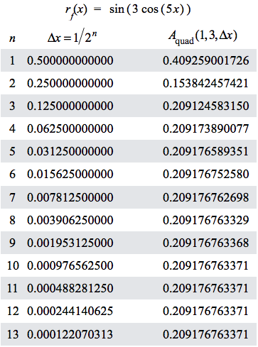
In Section 10.1 we examined different methods to approximate values of an accumulation function. In doing this we looked at tables of approximate values of $A_\mathrm{mid}(a,x,\Delta x)$ and $A_\mathrm{quad}(a,x,\Delta x)$ in relation to values of $\Delta x$ to inspect how their values converged for specific values of $a$ and x as we made values of $\Delta x$ smaller.

Figure 10.2.0 shows a table of values like we saw in Section 10.1. The first column contains values of $n$. The second column contains values of $\Delta x=1/2^n$. The third column contains values of $A_\mathrm{quad}(1,3,\Delta x)$.

Figure 10.2.0. Table of values for $n$, $\Delta x=1/2^n$, and $A_\mathrm{quad}(1,3,\Delta x)$.

Figure 10.2.0 gives us information about how values of $A_\mathrm{quad}(1,3,\Delta x)$ behave as $\Delta x$ becomes smaller. We can also look at the values of $A_\mathrm{quad}(1,3,\Delta x)$ in relation to values of $n$. Taking values of $A_\mathrm{quad}(1,3,\Delta x)$ in relation to values of $n$ makes what we will call a sequence.

Sequences

A sequence is an ordered list of numbers. It is sometimes called an indexed list. Each number in the list is indexed by its ordinal position in the list.

Another way to state this is that a sequence is a function from a subset of $\mathcal{N}$, the set of natural numbers $\{1, 2, 3, \cdots\}$, to the real numbers.

When the subset of $\mathcal{N}$ contains numbers from 1 to some definite number, the sequence is finite. When the subset is all of $\mathcal{N}$, the sequence is infinite.

The function f defined as $f(n)=2n-1, n \in \mathcal{N}$ produces the sequence $\left\langle f(1), f(2), f(3), \cdots \right\rangle=\left\langle 1, 3, 5, \cdots\right\rangle$. The symbol "$\in$" means "in" or "is an element of".

The function that maps natural numbers to the reals in Figure 10.2.0 is $n\mapsto A_\mathrm{quad}(1,3,1/2^n)$, or $f(n)=A_\mathrm{quad}(1,3,1/2^n),\, n\in \mathcal{N}$.

The terms in a sequence need not follow a pattern. The list $\langle 2, 45, 30, 77, 37, 88, 100, 65\rangle$ in pointed brackets is a sequence simply because its terms are ordered. The list's 1$^\text{st}$ term is 2, its 2$^\text{nd}$ term is 45, its 3$^\text{rd}$ term is 30, and so on. The pointed brackets are used to indicate that the list is ordered. If you change term's order in a sequence, then you've made a different sequence.

The difference between a set of terms and a sequence of terms is more easily understood by a shopping example.

If on a shopping trip you write a reminder to get sugar, flour, peanut butter, Pepsi, coffee, almond milk, and cereal, and you care only that you walk out of the store with these items, then you are thinking of a set of items. The order in which you put items into your basket doesn't matter to you.

However, if you write your reminder so that items in it reflect an efficient route among the store's isles, then varying the order of items in your list changes the route you'll take within the store. Your reminder is a sequence. The order in which you write the items in it matters in regard to the order in which you get them.

Another convention is to represent a list with a general term and an index, such as $\langle a_i\rangle$. This notation hides the underlying function. Using function notation, we would write $\left\langle a(i)\right\rangle$. Often, you will need to use function notation to define a sequence when graphing it or making a table in GC.

We often represent terms in a sequence using a subscript as the term's index, such as $a_2$ to represent the $2^\text{nd}$ term in the sequence $\langle a_i\rangle$. This means the same thing as saying that we are talking about $a(2)$, where $a$ is a function defined on $\mathcal{N}$.

The index of a term tells its place in the list. The subscript "5" in $a_5$ tells us that this term is fifth in the list, which means that it is preceded in the list by four terms. The statement $a_5=37$ means that 37 is the $5^\text{th}$ term in the sequence $\langle a_i\rangle$. You could also mix notations, writing $a_5=a(5)$.

An infinite sequence is one that has no last term. A function defined on all of $\mathcal{N}$ is an infinite sequence.

The notation $$\left\langle s_i\right\rangle=\left\langle\frac{1}{2^i}\right\rangle_{i=1}^\infty$$represents an infinite sequence by stating the sequence's general term. This is a compact way to represent the infinite sequence $$\left\langle s_i\right\rangle=\left\langle\dfrac{1}{2^1},\dfrac{1}{2^2},\dfrac{1}{2^3},\, \cdots\right\rangle.$$It is also a shorthand for representing the same sequence with function notation: $$s(i)=\frac{1}{2^i}, i \in \{1, 2, 3, \cdots\}.$$

Reflection 10.2.1. Explain how $\left\langle b_i\right\rangle=\left\langle \dfrac{i}{i+1}\right\rangle_{i=1}^\infty$ and $b(i)=\dfrac{i}{i+1},\,i\in \{1, 2, 3, \cdots\}$ represent the same sequence.

Series

A series is the sum of the terms in a sequence.

The series made from the sequence $\langle a_i\rangle=\langle 2,45,30,77,37,88,100,65\rangle$ stated above is $$\begin{align}\sum\limits_{i=1}^8 a_i&=a_1+a_2+a_3+a_4+a_5+a_6+a_7+a_8\\[1ex]&=2+45+30+77+37+88+100+65\end{align}$$

Many textbooks reserve the word "series" for the sum of terms in an infinite sequence. We will use "series" more broadly, to cover a sum of terms in either a finite or infinite sequence. In our usage, an "infinite series" is a series created from an infinite sequence.

A partial sum is the sum of the first $n$ terms of a sequence. If $\left\langle s_i\right\rangle_{i=1}^\infty$ is an infinite sequence, then $S_n$, the $n^\text{th}$ partial sum, is $\displaystyle{\sum_{i=1}^n s_i}$, the sum of the first $n$ terms of the sequence.

The ideas of sequence and series can be mixed.You can create a sequence of partial sums from a sequence. A sequence of partial sums is just a list of sums of successively longer subsequences.

A sequence of partial sums $\left\langle S_i\right\rangle$ is made from a sequence $\left\langle s_i \right\rangle$ by making $S_k=\sum\limits_{i=1}^{k} s_i$.

For example, the sequence $\left\langle s_i\right\rangle=\left\langle\frac{1}{2^1},\frac{1}{2^2},\, \cdots\right\rangle$ can be turned into a sequence of partial sums $\left\langle S_i\right\rangle$ where the $k^\mathrm{th}$ term in $\left\langle S_i\right\rangle$ is $\displaystyle{S_k=\sum\limits_{i=1}^{k}\frac{1}{2^i}}$.

A statement like $\displaystyle{S_k=\sum\limits_{i=1}^{k}\frac{1}{2^i}}$ is called the general term of the sequence of partial sums.

Example of a sequence of partial sums:

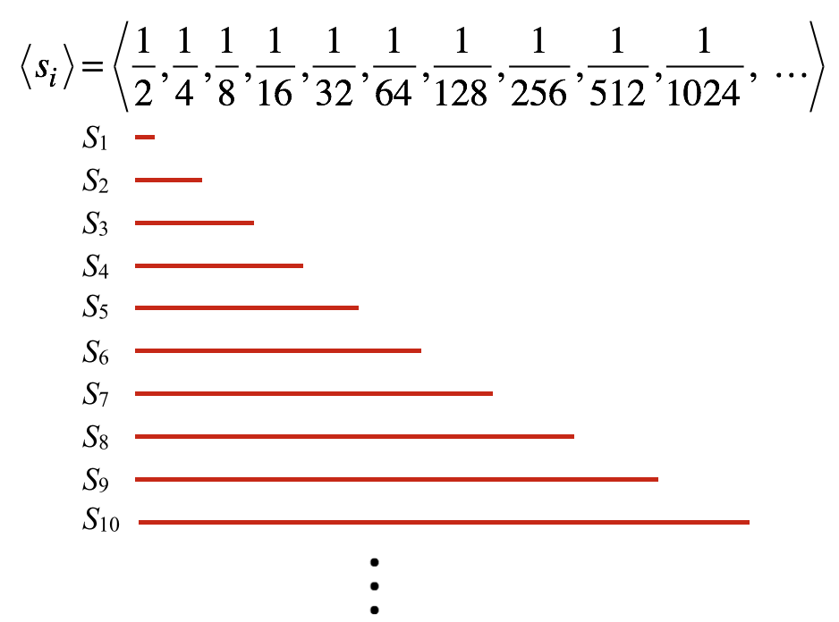
$$\begin{align} \text{Given: }\left\langle s_k\right\rangle_{k=1}^n &=\left\langle\dfrac{1}{2^1},\dfrac{1}{2^2},\dfrac{1}{2^3},\dfrac{1}{2^4},\, \cdots,\frac{1}{2^n}\right\rangle\text{, then}\\[1ex] \left\langle S_k\right\rangle_{k=1}^{n} &=\left\langle \sum\limits_{i=1}^{1}\frac{1}{2^i},\sum\limits_{i=1}^{2}\frac{1}{2^i},\sum\limits_{i=1}^{3}\frac{1}{2^i},\, \cdots,\sum\limits_{i=1}^{n}\frac{1}{2^i}\right\rangle \\[1ex] &=\left\langle \left( \frac{1}{2}\right),\left(\frac{1}{2}+\frac{1}{4}\right),\left(\frac{1}{2}+\frac{1}{4}+\frac{1}{8}\right),\left(\frac{1}{2}+\frac{1}{4}+\frac{1}{8}+\frac{1}{16}\right),\cdots,\left(\frac{1}{2}+\frac{1}{4}+\frac{1}{8}+\frac{1}{16}+\cdots+\frac{1}{2^n}\right)\right\rangle\\[1ex] &=\left\langle \frac{1}{2},\frac{3}{4},\frac{7}{8},\frac{15}{16},\frac{31}{32},\frac{63}{64},\, \cdots,\frac{2^n-1}{2^n}\right\rangle\end{align}$$

Figure 10.2.1 gives a way to visualize the construction of the sequence of partial sums shown above.

Figure 10.2.1. Constructing a sequence $\left\langle S_i\right\rangle$ of partial sums by adding the terms
in successively longer subsequences of the sequence $\left\langle s_i\right\rangle$.

Reflection 10.2.3. Rewrite the GC statement that you made for Reflection 10.2.2, but use function notation if you didn't use function notation originally.

Exercise Set 10.2.1

Practice writing the general term of a sequence. Hint: Write each term's index above the term. Also, your work in exercises 1-4 will be foundational for exercises 8-19.

1. Download this file. Define $s$ so that it produces this sequence:
   
   $\left\langle s_k\right\rangle=\left\langle 2, 4, 6, 8, 10, 12, 14, 16, 18, 20, 22\right\rangle$
2. Download this file. Define $s$ so that it produces this sequence:
   
   $\left\langle s_k\right\rangle=\left\langle 25, 16, 9, 4, 1, 0, 1, 4, 9, 16, 25\right\rangle$
3. Download this file. Define $s$ so that it produces this sequence:
   
   $\left\langle s_k\right\rangle=\left\langle 1.25, 2, 3.25, 5, 7.25, 10, 13.25, 17, 21.25, 26, 31.25\right\rangle$
4. Download this file. Define $s$ so that it produces this sequence:
   
   $\left\langle s_k\right\rangle=\left\langle 0, 6, 24, 60, 120, 210, 336, 504, 720, 990, 1320\right\rangle$

Practice with summation notation

5. Write $\displaystyle{\sum_{k=1}^{12} k(k+1)}$ without using summation notation. Leave terms in open form (uncalculated).
6. Write $\displaystyle{\sum_{k=1}^{6} r_f(a+(k-1)\Delta x)\Delta x}$ without using summation notation. Leave terms in open form (uncalculated).
7. Write $\displaystyle{\sum_{j=1}^{8} (j-1)!}$ without using summation notation. Leave terms in open form (uncalculated). Note: The notation $n!$ means $n(n-1)(n-2)\cdot \cdots\cdot 2\cdot 1$. We define 0! as $0!=1$.
8. Write 2 + 4 + 6 + 8 + 10 + 12 + 14 + 16 + 18 + 20 + 22 using summation notation.
   Enter your expression into GC (use ctrl-shift-S to get the summation symbol). GC should say that your sum is 132.
9. Write 25 + 16 + 9 + 4 + 1 + 0 + 1 + 4 + 9 + 16 + 25 using summation notation.
   Enter your expression into GC. GC should say that your sum is 110.
10. Write 1.25 + 2 + 3.25 + 5 + 7.25 + 10 + 13.25 + 17 + 21.25 + 26 + 31.25 using summation notation.
    Enter your expression into GC. GC should say that your sum is 137.5.
11. Write 0 + 6 + 24 + 60 + 120 + 210 + 336 + 504 + 720 + 990 + 1320 using summation notation.
    Enter your expression into GC. GC should say that your sum is 4290.

Practice with partial sums

12. Use GC to write the sequence of partial sums for the sequence in #1.
13. Use GC to write the sequence of partial sums for the sequence in #2.
14. Use GC to write the sequence of partial sums for the sequence in #3.
15. Use GC to write the sequence of partial sums for the sequence in #4.

Practice writing the general term of a sequence of partial sums. Write the geneal term in place of the blank on the right side.

16. Write the general term for the sequence of partial sums in #12: $\left\langle S_k\right\rangle=\left\langle \_\_\_\_\_\_\right\rangle$.


17. Write the general term for the sequence of partial sums in #13: $\left\langle S_i\right\rangle=\left\langle \_\_\_\_\_\_\right\rangle$.


18. Write the general term for the sequence of partial sums in #14: $\left\langle S_j\right\rangle=\left\langle \_\_\_\_\_\_\right\rangle$.


19. Write the general term for the sequence of partial sums in #15: $\left\langle S_q\right\rangle=\left\langle \_\_\_\_\_\_\right\rangle$.

Geometric Sequences and Series

Here are two examples of infinite geometric sequences:

$$\begin{align} a&=3, r=2\\[1ex] \left\langle b_i\right\rangle_{i=1}^\infty&=\left\langle 3\left(2^{i-1}\right)\right\rangle_{i=1}^\infty \\[1ex] &=\left\langle 3, 6, 12, 24, 48, \,\dots\right\rangle\\[1ex] \text{Notice that we could start the index at 0 to write }&\left\langle 3\left(2^{i-1}\right)\right\rangle_{i=1}^\infty\text{ as }\left\langle 3\left(2^i\right)\right\rangle_{i=0}^\infty\\[4ex] a&=2, r=\frac{2}{3}\\[1ex] \left\langle d_k\right\rangle_{k=1}^\infty &=\left\langle 2\left(\frac{2}{3}\right)^{k-1}\right\rangle_{k=1}^\infty\\[1ex] &=\left\langle 2\left(\frac{2}{3}\right)^0,2\left(\frac{2}{3}\right)^1,2\left(\frac{2}{3}\right)^2,2\left(\frac{2}{3}\right)^3,\,\dots\right\rangle\\[1ex] &=\left\langle 2, \frac{4}{3}, \frac{8}{9}, \frac{16}{27},\,\dots\right\rangle\\[1ex] \text{Notice that we could start the index at 0 to write }&\left\langle 2\left(\frac{2}{3}\right)^{i-1}\right\rangle_{i=1}^\infty\text{ as }\left\langle 2\left(\frac{2}{3}\right)^i\right\rangle_{i=0}^\infty \end{align}$$

An infinite geometric series is therefore of the form:

$$a\sum_{i=1}^\infty r^i$$where $\left\langle ar^j\right\rangle_{j=1}^\infty$ is a geometric sequence.

The sequence of partial sums made from an infinite geometric sequence is therefore $$\left\langle a\sum_{i=1}^j r^i\right\rangle_{j=1}^\infty$$where $\left\langle ar^k\right\rangle_{k=1}^\infty$ is a geometric sequence.

Reflection 10.2.4. The first three partial sums for $\left\langle 2\left(\frac{2}{3}\right)^i\right\rangle_{i=0}^\infty$ are:$$\begin{align} S_1&=2\left(\frac{2}{3}\right)^0\\[1ex] S_2&=2\left(\frac{2}{3}\right)^0+2\left(\frac{2}{3}\right)^1\\[1ex] S_3&=2\left(\frac{2}{3}\right)^0+2\left(\frac{2}{3}\right)^1+2\left(\frac{2}{3}\right)^2 \end{align}$$Write the next three partial sums. Use GC and summation notation to evaluate $S_1$ through $S_6$.

Defining Geometric Sequences and Series Recursively

The k^th term of a geometric sequence is $s_k=ar^k$ for $a,r\neq 0$. When we write $ar^k$ as $ar^k=r\left(ar^{k-1}\right)$, we see that $s_k=rs_{k-1}$. Defining the general term of a sequence in relation to the term or terms preceding it is called a recursive definition. Also, in defining a sequence recursively we must state the value of the first term so that the process stops.

Define the sequence $\left\langle s_k\right\rangle$ by the general term $s_k=0.7 s_{k-1}$ and $s_1=3$.

Then $s_{10}$ is $0.7s_9$, $s_9$ is $0.7 s_8$, and so on: $$\begin{align} s_{10} &= 0.7 s_9\\[1ex] &= 0.7(0.7 s_8)\\[1ex] &= 0.7(0.7 (0.7 s_7)\\[1ex] &= \cdots \\[1ex] &= 0.7(0.7 (0.7 (0.7 \cdots (0.7s_1))))\\[1ex] &= 0.7(0.7 (0.7 (0.7 \cdots (0.7\cdot 3))))\\[1ex] &= 3 \cdot 0.7^9 \end{align}$$

You can use GC to define sequences recursively. Figure 10.2.Insert is a recursive definition of the sequence with general term $s_k=0.75 s_{k-1}$ and $s_1=2$.

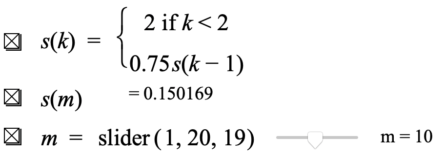
Figure 10.2.Insert A recursive definition of $s_k=0.75s_{k-1}$ and $s_1=2$. Click here to download the GC file.

A famous series defined recursively

Start with the interval $[0,1]$. Color the middle 1/3 without its endpoints, leaving the closed intervals $\left[0,\frac{1}{3}\right]$ and $\left[\frac{2}{3},1\right]$ uncolored. Now color the middle thirds of the remaining intervals without their endpoints, leaving the closed intervals $\left[0,\frac{1}{9}\right]$, $\left[\frac{2}{9},\frac{1}{3}\right]$,$\left[\frac{2}{3},\frac{7}{9}\right]$, and $\left[\frac{8}{9}, 1\right]$ uncolored. Keep going. (See Figure 10.2.2)

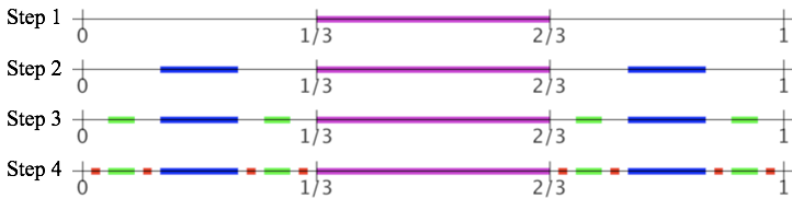
Figure 10.2.2. At each step, color middle thirds of uncolored intervals.

What is the combined lengths of the colored intervals after the 4^th step? The 15^th step?

Analysis of removing middle thirds

At each step, we color 1/3 of the length of uncolored intervals. So the combined lengths of colored intervals at step $k$ is the combined lengths at step $(k-1)$ plus 1/3 of the uncolored lengths. But the combined length of the uncolored intervals at step $(k-1)$ is 1 - colored lengths at step $(k-1)$.

Figure 10.2.3 shows a GC file that implements this solution.

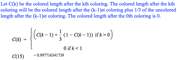
Figure 10.2.3. A solution to the colored interval problem.

The function $C$ as defined in Figure 10.2.3 is computationally inefficient. It takes about 12 seconds on a 6-core 2.9gh Intel Core i9 laptop to compute $C(25)$. Simple algebra increases computational efficiency immensely (see Figure 10.2.4 and this GC file.)

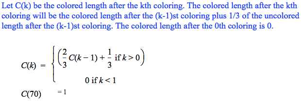
Figure 10.2.4. A more efficient GC solution to the colored interval problem.

The "color middle third" example produces a set of numbers called The Cantor Set. The Cantor Set has remarkable properties that you will study in a real anaysis course. One surprising property is that the set of numbers remaining (e.g., 1/9, 1/3, 2/3) is just as large as the set of numbers in the interval $[0,1]$ even though the combined lengths of colored intervals is essentially the length of the interval $[0,1]$.

Exercise Set 10.2.2

1. Let $a=1.5$ and $r=0.5$.
1. Write the first 10 terms of the geometric sequence in open form. Do not evaluate them.
2. Write the first 10 partial sums of this geometric sequence in open form. Use summation notation. Do not evaluate the partial sums.
3. Use this file to generate values of the first 20 partial sums from this sequence.
4. Write the values of $S_{38},\,S_{39},$ and $S_{40}$ to 12 significant digits.
2. Let $a=100$ and $r=1.025$.
1. Write the first 10 terms of the geometric sequence in open form. Do not evaluate them.
2. Write the first 10 partial sums of this geometric sequence in open form. Use summation notation. Do not evaluate the partial sums.
3. Use this file to generate values of the first 20 partial sums from this sequence.
4. Write the values of $S_{46},\,S_{47},$ and $S_{48}$ to 12 significant digits.
3. Let $a=1$ and $r=0.9$.
1. Write the first 10 terms of the geometric sequence in open form. Do not evaluate them.
2. Write the first 10 partial sums of this geometric sequence in open form. Use summation notation. Do not evaluate the partial sums.
3. Use this file to generate values of the first 20 partial sums from this sequence.
4. Write the values of $S_{258},\,S_{267},$ and $S_{300}$ to 12 significant digits.
4. You have a 30 meter piece of string.
• Cut 10 meters and lay it straight.
• Now cut 5 meters and lay it straight, at the end of the first piece.
• Cut 2.5 meters and lay it straight, at the end of the second piece.
• Do this 100 times.
• How much string remains from the original piece? Or, if you run out of string, at what step do you run out?
5. Let $\left\langle s_j\right\rangle$ be a sequence where $s_k=0.9 s_{k-1}$ and $s_1=2$.
1. Define a recursive function $s$ in GC that will compute $s(k)$ for any integer value of $k,\,k>0$.
2. In a new file, define a non-recursive, closed form function $s$ in GC that will compute $s(k)$ for any integer value of $k,\,k>0$.
3. Have GC compute $s(200)$ in each file. Which definition is computationally more efficient? Why?
6. In 1980, Aunt Hazel deposited $150 into a bank account and didn't touch it for 30 years. On each anniversary of her deposit, the bank added 8% of the current balance to her account.
1. What was Hazel's balance at the end of each year?
2. Use GC to generate a graph of Hazel's bank balance at each moment in time during those 30 years. Remember, the bank deposits interest at the end of each year.

7. Uranium 235 has a half life of approximately 700 million years. This means that x kilograms of uranium 235 will become $x/2$ kg of uranium 235 in 700 million years.

   According to the World Nuclear Association, there remains an estimated 5,718,400,000 kg of uranium 235 as of the year 2000.

   1. Assuming this figure is accurate, approximately how much uranium 235 existed 4.5 billion years ago?
   2. How much uranium 235 will be on earth in 75 billion years? (Just kidding. The sun will expand and absorb the earth long before then.)

Convergence and Divergence

The most important question we ask about an infinite series is whether it converges--whether terms in its sequence of partial sums become essentially indistinguishable. Most times we will be unable to answer that question directly. Instead, we will say whether a sequence of partial sums converges or does not converge by comparing it to one that we know converges or that we know fails to converge.

An infinite sequence converges if all terms after some place in the sequence become essentially indistinguishable from each other.

An infinite sequence diverges if it does not converge.

An infinite series converges if its sequence of partial sums converges.

An infinite series diverges if its sequence of partial sums diverges.

Reflection 10.2.6. Use function notation in saying what it means that an infinite sequence converges.

The phrase "become essentially indistinguishable from each other" is a matter of context and purpose. You might think at first that terms of a sequence are essentially indistinguishable if they agree to 15 decimal places. Later, you might decide that terms must agree to 22 decimal places before you consider them to be essentially indistinguishable from each other.

We must say that while our criterion for convergence, that terms in a sequence become "essentially indistinguishable from one another", worked well for us up to this moment, it was largely because we worked with integrals over finite intervals. We shall soon see that that we must think more carefully about what we mean that terms in a sequence become essentially indistinguishable from one another.

Harmonic Sequence and Series

The sequence $\left\langle\frac{1}{k}\right\rangle_{k=1}^\infty$ is a harmonic sequence and the sum $\sum_{j=1}^\infty\frac{1}{j}$ is a harmonic series. The name "harmonic" comes from the mathematics of musical harmony.

The harmonic series is important because many series can be compared to it easily to show that they diverge. The next section explains this.

That the harmonic series diverges seems counterintuitive. The term $1/j$ approaches 0 as $j$ becomes arbitrarily large! We eventually add successive terms that are essentially 0!

The divergence of the harmonic series $\sum_{j=1}^\infty \frac{1}{j}$ can be demonstrated in several ways. Figure 10.2.5 shows one. We compare each term in $\left\langle\frac{1}{j}\right\rangle_{j-1}^\infty$ to a term in another sequence which is less than or equal to it, and the infinite series made from the second sequence clearly diverges.

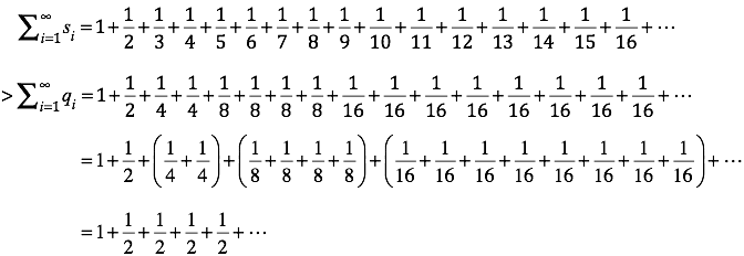
Figure 10.2.5. Each term $\left\langle s_i\right\rangle$ in this harmonic series is greater than or equal to a corresponding term in the sequence $\left\langle q_i\right\rangle$ such that $s_i\ge q_i$ and $\sum_{i=1}^\infty q_i$ diverges.

The harmonic series diverges slowly

The harmonic series' sequence of partial sums $\left\langle S_k\right\rangle=\left\langle\sum_{j=1}^k\frac{1}{k}\right\rangle$ diverges quite slowly. We can see this by looking at the number of terms to make successive sums of 1/2 in the last line of Figure 10.2.5

In Figure 10.2.5, it takes 2 terms with denominator 4 to make a sum of 1/2, 4 terms with denominator 8 to make a sum of 1/2, and 8 terms with denominator 16 to make a sum of 1/2. In general, it takes $2^{n-1}$ terms with denomiator $2^n$ to make a sum of 1/2. So, for example, it will take 524,288 terms with denominator 1,048,567 to make a sum of 1/2.

We can use the identity $\sum\limits_{j=1}^n 2^{j-1}=2^n-1$ to compute the values of $n$ in $\left\langle\sum\limits_{j=1}^n q_j\right\rangle$ that make sums of 2, 2.5, 3, 3.5, and so on. Figure 10.2.6 shows that for $\left\langle\sum\limits_{j=1}^n q_j\right\rangle$ to make a sum of 4 we need 6 one-halfs to make a sum of 3, which requires $2^6-1=63$ terms. So $\sum\limits_{j=1}^{64} q_j = 4$.

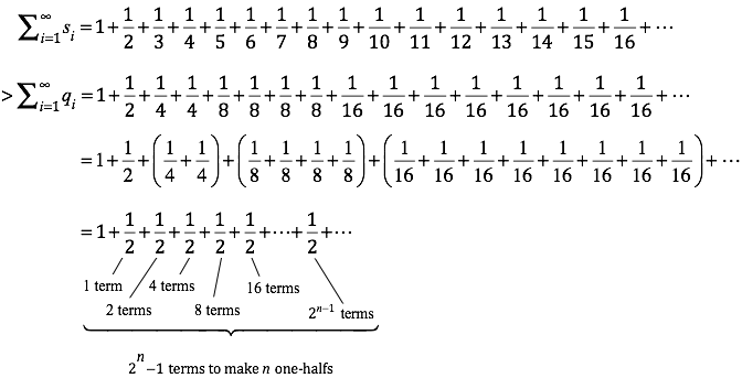
Figure 10.2.6. The series $\sum\limits_{i=1}^n q_i$ requires $2^n$ terms to produce a sum of $1+n/2$.

So, $\left\langle\sum\limits_{j=1}^n q_j\right\rangle=4$ when $n=64$. Likewise, $\left\langle\sum\limits_{j=1}^n q_j\right\rangle=7$ when $n=2^{12}=4096$ and $\left\langle\sum\limits_{j=1}^n q_j\right\rangle=9$ when $n=2^{16}=65,536$.

In general, the sequence $\left\langle\sum\limits_{j=1}^n q_j\right\rangle$ requires as many terms to produce an increase by 1/2 as the number of terms required to make the number of 1/2's already made.

Geometric series converge under some conditions and diverge under others

A geometric series is of the form

Graphing sequences

At the end of Section 10.1, we created a table of values to inspect whether $A_\mathrm{quad}(1,3,\Delta x)$ converged as $\Delta x$ became smaller. Figure 10.2.1 does the same thing, but does it in a way that creates sequences of values. The first column, labeled n lists integers from 1 to 20, in order. The second column, labeled $\Delta x=1/{2^n}$, lists values of $\Delta x$ that are created from values of n. The third column lists values of $A_\mathrm{quad}(1,3,\Delta x)$ that correspond to values of $\Delta x$.

We can consider each list as a sequence.

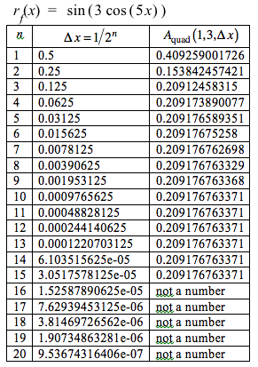
Figure 10.2.7. Using a table to create the sequences $\left\langle n_i\right\rangle=\left\langle i \right\rangle,\, \left\langle \Delta x_i\right\rangle=\left\langle\dfrac{1}{2^{n_i}}\right\rangle\text{, and }\left\langle A_i\right\rangle=\left\langle A_\mathrm{quad}(1,3,\Delta x_i\right\rangle$. The entries "not a number" are due to $\Delta x_i$ becoming so small that the computations exceed the capacity of the computer's 64-bit operating system.

Assuming that you have defined $A_\mathrm{quad}$ and its auxiliary functions, you can use GC to graph the values of $A_\mathrm{quad}(1,3,\Delta x_k)$ in relation to $x=3$ for $k=1$ to $k=100$ by typing the statement in Equation 10.2.1

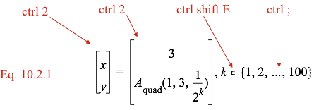
which produces the graph in Figure 10.2.8.

Figure 10.2.8. GC's plot of points $(3, A_\mathrm{quad}(1,3,1/k))$ for $k\in\{1, 2, \cdots,100\}$.

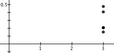
Figure 10.2.8's plot of points associated with $(3, A_\mathrm{quad}(1,3,1/k))$ for $k\in\{1, 2, \cdots,100\}$ is not very useful for visual inspection. The plotted points overlap, and we cannot tell which point goes with which value of $k$. We can resolve that problem easily by plotting $A_\mathrm{quad}(1,3,1/k))$ against values of $k$, as in Figure 10.2.10.

Figure 10.2.10. Values of $(3, A_\mathrm{quad}(1,3,1/k))$ plotted agains values of k, $k\in\{1,2,\cdots,100\}$.

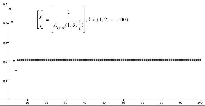
 Figure 10.2.10 suggests that the sequence $\left\langle A_k\right\rangle$=$\left\langle A_\mathrm{quad}(1,3,1/k)\right\rangle$ converges quickly so that all terms past $A_5$ appear essentially indistinguishable. However, this is merely a matter of scale.

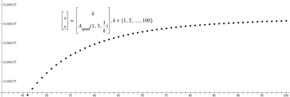
The sequence in Figure 10.2.4, magnified vertically around the points $(k,A_\mathrm{quad}(1,3,1/k)$ for $k=45$ to $k=100$ (Figure 10.2.11), shows otherwise. At the level of vertical magnification in Figure 10.2.11, values of $A_\mathrm{quad}(1,3,1/k)$ are clearly distinguishable. We shall revisit this issue in the next section when we take a closer look at the idea of convergence.

Figure 10.2.11. A closer look at values of $A_\mathrm{quad}(1,3,1/k)$ in relation to values of $k\in \{45, 46, \cdots, 100\}$.

(Do the same with geometric sequence and harmonic sequence)

Convergence (revisited)

(Fragmentary thoughts)

(A sequence converges if given any level of vertical magnification, there is a place in the sequence where all terms past that one are essentially indistinguishable. State this using index notation and function notation. Use figures from class lectures that show a window height as epsilon.)

(Consider the function $r_f$ defined as $r_f(x)=1+1/3^x$, where x varies through the real numbers greater than or equal to 1. Think of the sequence $f(n)=1+1/3^n$ as an approximate rate of change function with $\Delta x=1$. [Graph]. A series is like an accumulation function that has the sequence as its rate of change function that is constant over $\Delta x$-intervals of length 1. [Graph]. We can  compare the sum of the sequence to the integral.

If f is a decreasing function, f(x)>0, use the right method to compare the series with the integral of f. If the integral of f has a limit, the series has a limit.

Think of necessary conditions for convergence of a sequence's series. For sure, terms must become essentially equal to 0.