| < Previous Section | Home | Next Section>> |
Until now we have used "parameter" to mean a letter that stands for a value that is constant within a specific situation but can have different values in different situations. A classic example of distinguishing parameters from variables is $y=mx+b$, the general represenation of a linear function. We consider values of $m$ and $b$ as fixed while values of x and y vary. But $m$ and/or $b$ will have different values in different linear functions.
However, "parameter" has slightly different meanings in different disciplines. In science, "parameter" often means a fundamental quantity in a system by which all other quantities in the system can be related. For example, t is a parameter where "t" stands for elapsed time and all functions that define values of quantities in the system are expressed as functions of t. Values of quantities so defined can be related because they all occur at a common value of t.
Time need not be the fundamental quantity in a system. As we saw in Exercise 12.0.1.8, the radius of a sphere can be thought of as a parameter in this second sense. Volume and surface area of a sphere can each be expressed as a function of the sphere's radius, so we can relate a sphere's volume and surface area by putting values of volume on one axis and values of surface area on the other axis. Vallues of volume and surface area were related because they occurred at the same radius. However, values of the radius did not appear on any axis.
Another way to think of parameters in the second sense is to imagine that coordinates of points on a graph are each functions of a third variable. Instead of a point having coordinates $(x,y)$ it has coordinates $(x(t),y(t))$. The x-coordinate of a point is a function of t and the y-coordinate of a point is also a function of t.
We will write relationships represented with the use of a parameter as $(x,y)=[x(t),y(t)]$. Represent such relationships in GC as you did in Section 12.0.
You already experienced coordinates being defined as functions of a third variable in Section 12.0. We had GC produce graphs that showed values of one quantity (e.g., volume of poured concrete at a moment in time) in relation to values of another quantity (e.g., rate of change of volume with respect to time). Volume and its rate of change were each defined as functions of elapsed time since the pouring chute opened. We related values of $f(t)$ and $r_f(t)$ by plotting their values against each other for common values of t.
A relationship between variables is defined parametrically when each variable is defined as a function of an additional, common variable. Sometimes the relationship describes one variable as a function of the other.
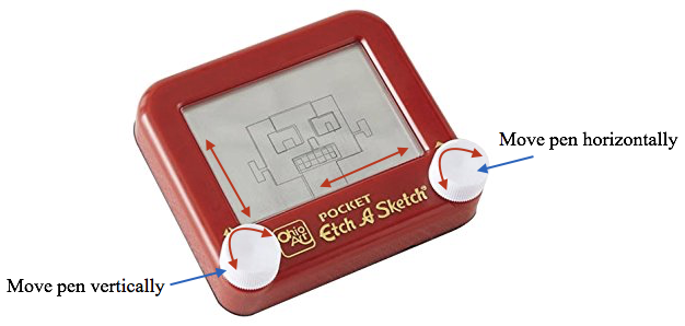
You can think of creating graphs parametrically as if you are programming an Etch A Sketch (Figure 12.1.1). Think of defining one function to control vertical movement of the Etch A Sketch's pen and program another function to control horizontal movement of the Etch A Sketch's pen.
Figure 12.1.1 You sketch figures with an Etch A Sketch by rotating dials. A "pen" leaves a trace on the screen in response to rotating the dials. One dial moves the pen vertically; the other moves the pen horizontally. Rotating dials simultaneously produces slanted lines. Rotating one dial at varying angular velocities while rotating the other at a constant angular velocity produces curves.
For example, consider the graph in Figure 12.1.1. We can envision it in terms of the x-coordinate being a function of t and the y-coordinate being a function of t.
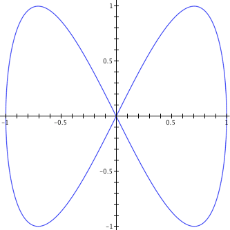
Figure 12.1.2.
Figure 12.1.3 illustrates a way to break down a curve into parts that give hints about a function that behaves like the x or y coordinate of the graph.
In other words, we can envision the graph emerging as the value of x varies from 0 to 1, then 1 to 0, then 0 to -1, then -1 to 0. What function has an output value that varies this way? The sine function! So we can try $x(t)=\sin(\text{something})$.
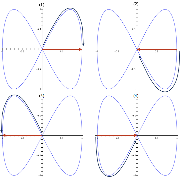
Figure 12.1.3.
Now focus on the y-coordinate of points on the graph as the value of x varies (Figure 12.1.4).
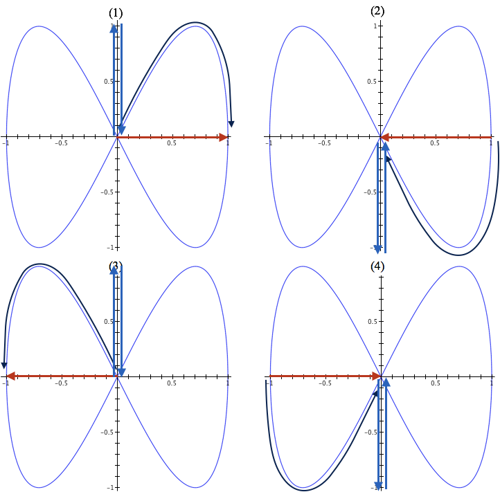
Figure 12.1.4.
What function has values that vary from 0 to 1 to 0 to -1 to 0 repeatedly? The sine function again! However, this sine function must have an argument that makes the value of sine cycle through a full period twice as fast as the argument that produces the horizontal coordinate. So we can try $y(t) = \sin(2\times\text{the argument for the x-coordinate})$.
If t varies from 0 to 1, then $2\pi t$ varies from 0 to $2\pi$, and $\sin(2\pi t)$ varies from 0 to 1 to 0 to -1 to 0 while $\sin(4\pi t)$ varies from 0 to 1 to 0 to -1 to 0 twice (see Figure 12.1.5).
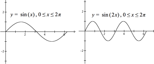
Figure 12.1.5.
Our guess at a way to make the graph in Figure 12.1.2 is then$$\left[\array{x \cr y}\right]=\left[\array{\sin(2\pi t) \cr \sin(4\pi t)}\right].$$
Test the above statement in GC to see if it generates the desired graph. Press "ctrl 2 = ctrl 2" to get $\left[\array{x \cr y}\right]=\left[\array{x \cr y}\right]$ and then replace x and y in the second matrix with appropriate expressions.
Reflection 12.1.1. Download and open this file. Answer questions in it.
We have seen several times that$$\left[\array{x \cr y}\right]=\left[\array{\sin(2\pi t) \cr \cos(2\pi t)}\right],\, 0\le t \le 1$$generates a circle of radius 1 centered at the origin.
It is easy to see that$$\left[\array{x \cr y}\right]=\left[\array{\sin(2\pi \sqrt t) \cr \cos(2\pi \sqrt t)}\right],\, 0\le t \le 1$$also generates a circle of radius 1 centered at the origin. Are the two graphs the same? The answer is "yes and no".
The two graphs contain the same set of ordered pairs. So, as sets of points, the two graphs are the same. But if we consider a point in relation to the value of t that produces that point, then the two graphs are not the same.
In Figure 12.1.6, the blue point is generated by $\left[\array{\sin(2\pi n) \cr \cos(2\pi n)}\right]$. The red point is generated by $\left[\array{\sin(2\pi \sqrt n) \cr \cos(2\pi \sqrt n)}\right]$ as the parameter n varies from 0 to 1. The red point initially moves faster along the circle than the blue point.
The graph on the right shows why: $\sqrt t \gt t$ for all values of t as t varies from 0 to 1, with the exception $\sqrt t=t$ at the moments $t=0$ and $t=1$.
Figure 12.1.6. Blue dot moves according to $t=u$. Red dot moves according to $t=\sqrt u$.
Figure 12.1.7 gives another perspective on how the two graphs are generated differently with respect to t.
Instead of suppressing t as in Figure 12.1.6, we represent values of t on the z-axis.
It should be clear from Figures 12.1.6 and 12.1.7 that the relationships $t\mapsto [\cos(2\pi t),\sin(2\pi t)]$ and $t\mapsto [\cos(2\pi \sqrt t),\sin(2\pi \sqrt t)]$ are not the same even though they both make a circle of radius 1 centered at the origin.
Figure 12.1.7.
The path of a moving object is called its trajectory. It is often useful to model an object's trajectory by imagining the object's position within a coordinate system and defining its coordinates as functions of a parameter.
Figure 12.1.8 depicts a planet orbiting a sun and a moon orbiting the planet. (Orbits are depicted here as circular even though actual orbits are slightly elliptical.)
The planet is 2 astronomical units (au) from its sun and the moon is 0.2 au from the planet. The planet orbits its sun once per year. The moon orbits the planet 7 times per year.
Figure 12.1.8. Simulation of a planet orbiting its sun and a moon orbiting the planet. The planet orbits its sun once per year. The moon orbits the planet 7 times per year.
The planet's trajectory around its sun is a circle of radius 2 au. The moon's trajectory around the planet is a circle of radius 0.2 au. What is the moon's trajectory around the sun?
We will model the planet's motion around its sun and the moon's motion around the planet parametrically. This will allow us to show the moon's trajectory around the sun.
In Exercises 4 and 5 of Section 12.0 you explained why $$\left[\array{x \cr y}\right]=c \left[\array{\sin(2\pi t) \cr \cos(2\pi t)}\right]=\left[\array{c\sin(2\pi t) \cr c\cos(2\pi t)}\right]$$ produces a circle of radius c with a clockwise orientation centered at $[0,0]$ for $0\le t\le 1$. The planet's position at the moment $t=n$ is $$\left[\array{x \cr y}\right]=2 \left[\array{\sin(2\pi n) \cr \cos(2\pi n)}\right]$$which will traverse the circle once as n varies from 0 to 1.
The moon's trajectory around the planet (taking the planet's position as the moon's origin) has a clockwise orientation, and is therefore $$\left[\array{x \cr y}\right]=0.2 \left[\array{\cos(2\pi t) \cr \sin(2\pi t)}\right]=\left[\array{0.2\cos(2\pi t) \cr 0.2\sin(2\pi t)}\right].$$
However, the moon traverses its trajectory 7 times as t varies from 0 to 1, so the moon's position relative to the planet at the moment $t=n$ is $$\left[\array{x \cr y}\right]=0.2\left[\array{\cos(7(2\pi n)) \cr \sin(7(2\pi n))}\right].$$
Notice that the coordinates $\sin(...)$ and $\cos(...)$ in the planet's trajectory are reversed in the moon's trajectory. This is because the planet's trajectory relative to its sun has a clockwise orientation while the moon's trajectory relative to the planet has a counter-clockwise orientation.
We have the planet's position relative to the sun and the moon's position relative to the planet. We now need the moon's position relative to the sun.
Figure 12.1.9 shows that
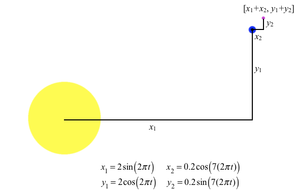
Figure 12.1.9. Determining the x- and y-coordinates of the moon relative to the sun.
The moon's trajectory relative to the sun is therefore $$\begin{align}\left[\array{x \cr y}\right] &=\left[\array{2\sin(2\pi t) \cr 2\cos(2\pi t)}\right]+\left[\array{0.2\cos(7(2\pi t)) \cr 0.2\sin(7(2\pi t))}\right]\\[1ex] &=\left[\array{2\sin(2\pi t)+0.2\cos(7(2\pi t)) \cr 2\cos(2\pi t)+0.2\sin(7(2\pi t))}\right]\end{align}$$
for $0\le t \le 1$, and the moon's position relative to the sun at the moment $t=n$ is$$\left[\array{x \cr y}\right]=\left[\array{2\sin(2\pi n)+0.2\cos(7(2\pi n)) \cr 2\cos(2\pi n)+0.2\sin(7(2\pi n))}\right]$$
Figure 12.1.10 shows the moon's trajectory relative to the sun.
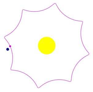
Figure 12.1.10 Trajectory of moon in relation to sun.
Reflection 12.1.4 leads you to investigate and understand all of the above.
Reflection 12.1.4 Download this file. Explain:
Use GC to graph the asteroid's trajectory around the sun.
All the relationships you worked with in Section 12.0 were defined parametrically. We just didn't say so. Some relationships between x-coordinates and y-coordinates defined x as a function of y or y as a function of x.
Until Chapter 12 we said that a relationship between y and x was a function if every value in the domain of x corresponded to exactly one value in the domain of y.
With our new ability to define relationships parametrically, we can inquire whether the relationship between t and $[x(t),y(t)]$ defines $[x(t),y(t)]$ as a function of t just as we can inquire whether the relationship between $y(t)$ and $x(t)$ defines one as a function of the other.
You explored a circle as the graph of $[\cos(2\pi t),\sin(2\pi t)],\,0\le t \le 1$ in Exercise 12.0.1.4. The value of $\cos(2\pi t)$ gave the x-coordinate of a point on the circle; the value of $\sin(2\pi t)$ gave the y-coordinate of the same point.
You also determined that the relationship $t\mapsto \left[\cos(2\pi t),\sin(2\pi t)\right],\,0\le t \le 1$ is a function. In GC the definition of p is$$p(t)=\left[\array{\cos(2\pi t) \cr \sin(2\pi t)}\right]$$and you would graph it by entering $$\left[\array{x \cr y}\right]=p(t)$$Every value of t corresponds to exactly one point on the circle. The fact that $p(0)$ and $p(1)$ are both $[1,0]$ is immaterial. The only thing that matters is that every value of t corresponds to exactly one point on the circle.
The function $t\mapsto \left[\cos(2\pi t),\sin(2\pi t)\right],\,0\le t \le 1$ can be represented also as $p(t)=[\cos(2\pi t),\sin(2\pi t)],\,0\le t\le 1$. The function $p$ takes a number from 0 to 1 as input. The output $p(t)$ is a coordinate pair that determines a point on the circle.
In general, there are only two ways that a mapping $t\mapsto [x(t),y(t)]$ will not be a function:
The first case happens at the moment one of $x(t)$ or $y(t)$ fails to be a function because it has two values for some value of t.. For example, suppose that $x(1)=1$ and $x(1)=2$. In this case, there would be two coordinate pairs $[x(1),y(1)]$ that correspond to $t=1$, namely $[1,y(1)]$ and $[2,y(1)]$.
The second case happens at the moment one of $x(t)$ or $y(t)$ is undefined for a value of t. Then, there is no coordinate pair that corresponds to that value of t.
Figure 12.1.11 illustrates the second case: $x(t)=3t$ is defined at $t=1$ but $y(t)=\dfrac{1}{t-1}$ is not defined at $t=1$. Thus, there is a value of $x(t)$ that does not correspond to a value of $y(t)$, so $[x(t),y(t)]$ is not a function of t because there is no coordinate pair that corresponds to $t=1$. On the other hand, if we omit $t=1$ from the domains of x and y, then $t\mapsto [x(t),y(t)],t\neq 1$ does define a function.
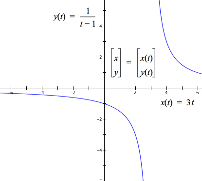
Figure 12.1.11. $x(1)$ is defined but $y(1)$ is undefined. Therefore, there is no pair $[x(t),y(t)]$ that corresponds to $t=1$.
We can focus on the conditions that guarantee $y(t)$ is a function of $x(t)$. Whatever we say for this case will apply to the case of $x(t)$ being a function of $y(t)$.
There are only two ways that $y(t)$ can fail to be a function of $x(t)$:
The first case means that there some value of $x(t)$ for which there is is no value $y(t)$ that corresponds to it.
The second case means that there are two values of $y(t)$ that correspond to a single value of $x(t)$. This happens at the moment $x(t)$ both increases and decreases as t varies and $y(t)$ is non-constant.
Figure 12.1.12 illustrates the second case: x is not a function of y because $x(-1)=x(1)=1$ but $y(-1)\neq y(1)$. That is, there is a value of $x(t)$ (namely, $x(t)=1)$ that corresponds to two values of $y(t)$, namely $y(t)=-3$ and $y(t)=3$. Therefore, $y(t)$ is not a function of $x(t)$. (Notice, though, that $x(t)$ is a function of $y(t)$.)
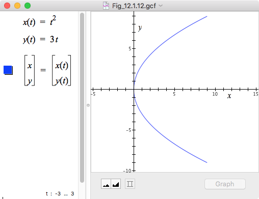
Figure 12.1.12. y(t) is not a function of x(t) because at least one value of $x(t)$ corresponds to more than one value of $y(t)$. On the other hand, x(t) is a function of y(t) because every value of $y(t)$ corresponds to exactly one value of $x(t)$.
Reflection 12.1.5. When considering whether $y(t)$ is a funciton of $x(t)$, why does it not matter that $x(t)=1$ for two different values of t but it matters that two values of $y(t)$ correspond with $x(t)=1$?
Reflection 12.1.6. Imagine the graph in Figure 12.1.11 being generated as t varies from -3 to 3. Track values of $x(t)$ and values of $y(t)$ as in Figure 12.0.3. Then explain how $y(t)$ fails to be a function of $x(t)$.
Figure 12.1.12 displays a graph of the relationship $\left[\array{x \cr y}\right]=\left[\array{t^2 \cr 3t}\right]$. The relationship between x and y is tacit; it is not represented explicitly.
It is sometimes desirable to transform a parametric representation of a relationship into a relationship represented explicitly. In Figure 12.1.12 we have $x=t^2$ and $y=3t, -3\le t\le 3$. We can solve for x in terms of y by eliminating t. $$\begin{align}y&=3t\\[1ex]t&=y/3&\text{(solving for }t)\\[1ex]x&=t^2\\[1ex]x&=y^2/9&\text{(substituting for } t)\end{align}$$.
Reflection 12.1.7. Use GC to confirm that $x=y^2/9,-9\le y\le 9$ and $\left[\array{x \cr y}\right]=\left[\array{t^2 \cr 3t}\right], -3\le t \le 3$ generate the same graph.
Set lower and upper values for t to $-3$ and 3, respectively, after graphing $\left[\array{x \cr y}\right]=\left[\array{t^2 \cr 3t}\right]$
Figure 12.1.13 displays a line segment with endpoints $(a,b)$ and $(c,d)$. How do we represent points on this graph parametrically? By using proportional reasoning.
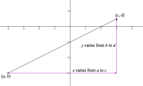
Figure 12.1.13. As x varies from a to c, y varies from b to d.
If we let t vary from 0 to 1, then we can represent the variation in x from a to b by $a+t(c-a)$. At the moment $t=0$, then $a+t(c-a)=a$. At the moment $t=1$, then $a+t(c-a)=c$. At the moment $0\lt t\lt 1$, then $a+t(c-a)$ is $100t$% of the way between a and c.
Similarly, at the moment $t=0$, $b+t(d-b)=b$ and at the moment $t=1$, $b+t(d-b)=d$. When $0\lt t\lt 1$ then $b+t(d-b)$ is $100t$% of the way between b and d.
We can represent variation along the line segment connecting $\left[\array{a \cr b}\right]$ and $\left[\array{c \cr d}\right]$ in parametric form as $$\begin{align} \left[\array{x \cr y}\right]&=\left[\array{a+t(c-a) \cr b+t(d-b)}\right]\\[1ex]&=\left[\array{a \cr b}\right]+\left[\array{t(c-a) \cr t(d-b)}\right]\\[1ex] &=\left[\array{a \cr b}\right]+\left[\array{tc-ta \cr td-tb}\right]\\[1ex] &=\left[\array{a \cr b}\right]+\left[\array{tc \cr td}\right]-\left[\array{ta \cr tb}\right]\\[1ex] &=\left[\array{a \cr b}\right]+t\left[\array{c \cr d}\right]-t\left[\array{a \cr b}\right]\\[1ex] &=(1-t)\left[\array{a \cr b}\right]+t\left[\array{c \cr d}\right]\end{align}$$
At the moment $t=0$, $(1-t)\left[\array{a \cr b}\right]+t\left[\array{c \cr d}\right]=\left[\array{a \cr b}\right]$.
At the moment $t=1$, $(1-t)\left[\array{a \cr b}\right]+t\left[\array{c \cr d}\right]=\left[\array{c \cr d}\right]$.
When $0\lt t \lt 1$, $(1-t)\left[\array{a \cr b}\right]+t\left[\array{c \cr d}\right]$ will be a point whose x- and y-coordinates change proportionally (the change in each being scaled by t) and will therefore lie on the segment connecting $\left[\array{a \cr b}\right]$ with $\left[\array{c \cr d}\right]$.
If we consider the line segment to be part of the graph of $f(x)=px+q$, with $(a,f(a))$ and $(b,f(b)$ being points on the graph, then $b=f(a)$ and $d=f(b)$ in the above derivation.
The parameterization of the graph of f is therefore $$\left[\array{x \cr y}\right]=(1-t)\left[\array{a \cr f(a)}\right]+t\left[\array{b \cr f(b)}\right]$$ where t takes on all the values in the domain of f.
The equation $\left[\array{x \cr y}\right]=(1-t)\left[\array{a \cr f(a)}\right]+t\left[\array{b \cr f(b)}\right]$ is called the parameterization of a line.
Reflection 12.1.8. Let $f(x)=0.5x-1$. Use GC to confirm that the graph of $\left[\array{x \cr y}\right]=(1-t)\left[\array{a \cr f(a)}\right]+t\left[\array{b \cr f(b)}\right],\,0\le t\le 1$, coincides with the graph of $y=f(x)$ for any values of a and b.
The method of parameterizing a line can be used to transform any shape into any other shape as long as the shapes can be represented parametrically.
Figure 12.1.14 presents a simple example. It shows the graph of $y=\sin(x)$ being transformed into the graph of $y=\sin(2x)e^{\cos 3x}$.
Figure 12.1.14 The graph of $y=\sin(x)$ morphs into the graph of $y=\sin(2x)e^{\cos(3x)}$ by parameterizing
segments connecting points $\left[\array{t \cr \sin(t)}\right]$ and $\left[\array{t \cr \sin(2t)e^{\cos(3t)}}\right]$.
The first loop of the animation (repeated twice) shows the graph of $y=f(x)$ morphing into the graph of $y=g(x)$. The second loop of the animation (repeated twice) illustrates how GC accomplishes the morph. It parameterizes segments connecting the points $\left[\array{t \cr f(t)}\right]$ and $\left[\array{t \cr g(t)}\right]$ for every value of t.
The GC file that made Figure 12.1.14 is here.
Reflection 12.1.9. Notice that we used two different types of parameters in the boxed statement. We used n as a parameter in the old sense, as a letter that stands for a constant that can be different in different situations. Different values of n determine different graphs.
We used the letter t with the new meaning of parameter, as a common variable in the definitions of two functions that define the coordinates of a set of points.
Reflection 12.1.10. Let $f(x)=x^2$ and $g(x)=\dfrac{\sin(x)}{x}$.
Confirm the claim stated in the black box. Show that for $n=0.25$, the points generated by $(1-n)\left[\array{k \cr f(k)}\right]+n\left[\array{k \cr g(k)}\right]$ are 25% of the way between $f(k)$ and $g(k)$ for $k\in \{0.1, 0.5, 0.75\}$.
| < Previous Section | Home | Next Section>> |