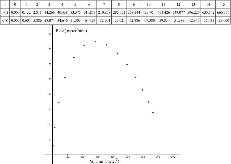
Figure 12.0.2. Collect corresponding values of $r_v(t)$ and $V(t)$ for values of t. Then plot the correspondence points $\left(V(t),r_v(t)\right)$.
| < Previous Section | Home | Next Section> |
In prior chapters we defined functions that gave information about the value of one quantity with respect to the value of another directly.
We asked, for example, how far an object has traveled after some number of seconds have elapsed when given the object's rate of change of distance with respect to time.
The accumulation function we defined in terms of the object's rate of change with respect to time allowed us to answer questions about the object's distance traveled at any moment in time.
There are other questions that arise naturally in such situations that cannot be answered so directly. For example:
We have a function for a car's velocity at each moment in time since it began moving. What was the car's velocity at every distance it traveled?
The difficulty we meet in answering this question is that we have distance as a function of time and velocity as a function of time, but we do not have velocity as a function of distance.
Cement is being poured into a building's foundation at the rate of $r_v(t)=t^4e^{-t/2}\text{ m$^3$/min}$ t minutes after the pouring chute opened. At what rate is cement being poured when $V\text{ m$^3$}$ of cement has been poured?
The cement's rate of change of volume with respect to time after t minutes is $r_v(t)=t^4e^{-t/2}\text{ m$^3$/min}$; its volume after t minutes is $\displaystyle{V(t)=\int_0^t r_v(u)du}\text{ m$^3$}$.
Normally, to express $r_v$ in terms of $V$ we would express t in terms of $V$, then substitute the resulting expression for t in the definition of $r_v(t)$. As you will see, we run into difficulties with this approach.
We can use integration by parts repeatedly to define $V(t)$ in closed form. We get $$\begin{align} V(t)&=\int_0^t u^4e^{-u/2}du\\[1ex] &=-2e^{t/2}\left(t^4+8t^3+48t^2+192t+384\right)+768. \end{align}$$
It will be daunting to express t in terms of $V$ when $V=-2e^{-t/2}\left(t^4+8t^3+48t^2+192t+384\right)+768$.
However, we can use GC to take a graphical approach. We can command GC to produce a graph of $r_v(t)$, the rate of change of poured concrete's volume with respect to time, in relation to $V(t)$, the concrete's volume with respect to time.
The idea will be to put values of $V(t)$ on the horizontal axis and values of $r_v(t)$ on the vertical axis. We can then inspect the graph for values of $r_v(t)$ that correspond to values of $V(t)$.
Figures 12.0.1, 12.0.2, and 12.0.3 show three stages in envisioning a graph of values of one function in relation to values of another function when they share a common argument.
Coordinating values of $r_v(t)$ and $V(t)$
Both $r_v(t)$ and $V(t)$ have a value for each value of t. We can put these values in relation to each other by plotting one on the horizontal axis and one on the vertical axis in a rectangular coordinate system.
Figure 12.0.1. To sketch a graph of $r_v(t)$ in relation to $V(t)$, do this repeatedly:
(1) Select a value of t;
(2) Determine values of $r_v(t)$ and $V(t)$;
(3) Place the value of $V(t)$ on the horizontal axis;
(4) Place the value of $r_v(t)$ on the vertical axis;
(5) Plot the correspondence point $\left(V(t),r_v(t)\right)$.
Collecting values in a table
Figure 12.0.1 illustrated the process of relating values of $r_v(t)$ in relation to $V(t)$. We can speed up this process by listing corresponding values of $r_v(t)$ and $V(t)$ in a table and plot points with these coordinaes in a rectangular coordinate system.
Figure 12.0.2. Collect corresponding values of $r_v(t)$ and $V(t)$ for values of t. Then plot the correspondence points $\left(V(t),r_v(t)\right)$.
Coordinating values of $r_v(t)$ and $V(t)$ as the value of t varies smoothly
Once we have the process of relating values of $r_v(t)$ and $V(t)$ in a coordinate system firmly in mind, we can imagine both values varying smoothly with t while relating them within a rectangular coordinate system.
Figure 12.0.3. Values of $r_v(t)$ and $V(t)$ vary as t varies. We coordinate values of $r_v(t)$ and $V(t)$ by imagining the
value of $r_v(t)$ varying on the vertical axis as the value of $V(t)$ varies on the horizontal axis.
Reflection 12.0.1. Describe how Figures 12.0.1, 12.0.2, and 12.0.3 give complementary information.
The graph of $r_v(t)$ in relation to $V(t)$ allows us to approach the question of how fast concrete is being poured when $V$ $\text{ m$^3$}$ of concrete has been poured. Figure 12.0.4 shows the point $(547.437,51.6719)$ highlighted on the graph of $r_v$ in relation to $V$. This means that when the volume of concrete is 545.53 $\text{ m$^3$}$ the volume is varying at the rate of 51.9871 $\text{ m$^3$/min}$.
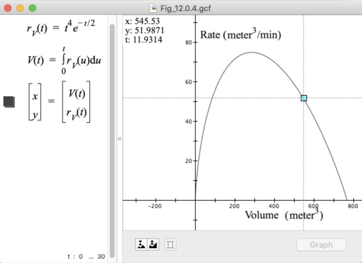
Figure 12.0.4. The concrete's volume is varying at 51.9871 $\text{ m$^3$/m}$ when its volume is 545.53 $\text{ m$^3$}$.
GC gives the additional information that this happened at $t=11.9314$ minutes.
Using GC to graph values of one function in relation to values of another
Figure 12.0.5 explains what to type in GC to generate Figure 12.0.4.
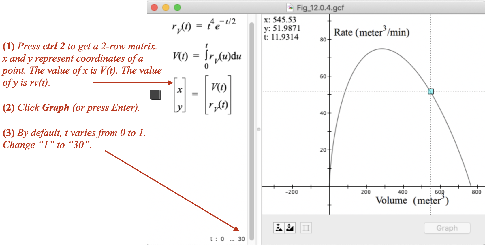
Figure 12.0.5. The GC file that created Figure 12.0.4.
Define $r_v$ and $V$. Then type ctrl 2 = ctrl 2 to get two 2-row by 1-column arrays separated by an equal sign.
In the second (right) array, replace x by $V(t)$ and y by $r_v(t)$.
Notice: In GC, the value of t varies from 0 to 1 by default. Press the Graph button, then change the upper value of t from "1" to "30".
Changing the range for t in GC is advisable only when you are graphing a single relationship, or when all relationships rely on t having the same range of values. When different relationships rely on t having different ranges of values it is better to leave the range of t as $0\dots 1$ and adjust functions' arguments accordingly. See Figure 12.0.5
On paper, you can use any variable as a parameter when defining parametric relationships. Unfortunately, GC requires you use t when defining a relationship parametrically. Moreover, the only way you may use "t" in a GC statement is to define a relationship parametrically.
Section 12.1 will refer back to Exercises 4 and 5, so attend to them closely.
Why does the statement$$\left[\array{x \cr y}\right]=\left[\array{\cos(2\pi t)\cr \sin(2\pi t)}\right]$$produce a circle of radius 1 centered at the origin?
Hint: For each value of t, $\cos(2\pi t)$ is a point's x-coordinate and $\sin(2\pi t)$ is that point's y-coordinate. Show this in a diagram and then use Pythagoras' Theorem and the identity $(\sin\theta)^2+(\cos\theta)^2=1$ to conclude that every point with coordinates $[\cos(2\pi t),\sin(2\pi t)]$ is 1 unit from $[0,0]$.
The notation $t\mapsto [x(t),y(t)]$ is commonly used to denote a relationship between x and y parametrically. It means "values of t are mapped to ordered pairs $[x(t),y(t)]$".
Does the relationship $t\mapsto [\cos(2\pi t),\sin(2\pi t)],\,0\le t\le 1$ make the circle a function of t?
Put another way: Is any value of t mapped to more than one point on the circle? Does every point on the circle have a value of t mapped to it? If your answer is "no" to either question, the circle is not a graph of a function. If both answers are "yes", then the circle is the graph of a function from values of t to points on the unit circle.
Circles, when graphed parametrically, have orientations. The orientation of a circle is determined by the direction of a point $[x(n),y(n)]$ that moves along it as the value of n increases through the parameter's domain.
If the point moves clockwise as n increases, the circle has positive orientation. If the point moves counter-clockwise, the circle has negative orientation.
What are the orientations of the circles created in Part (a) of this exercise? Explain.
It is well known in physics that horizontal motion and vertical motion are independent in a gravitational field.
This can be illustrated by an experiment where a bean bag is shot horizontally at the same moment an object is released from the same height as the bean bag.
The two will collide if they don't hit the ground first -- regardless of the bag's horizontal speed and regardless of the distance between bag and object. (See animation below.)
| < Previous Section | Home | Next Section> |