| < Previous Section | Home | Next Section > |
A central idea in calculus is to quantify relationships between quantities' values as they vary through small intervals.
However, it is sometimes counter-intuitive to anticipate a quantity's value varying through a large interval by varying smoothly through tiny intervals that compose it.
An activity might make the centrality of anticipating variation over small intervals more real to you. Please complete Activity 1.4.1 before returning to this page. It will be convenient for you to print this page first.
We hope Activity 1.4.1 conveyed two messages to you:
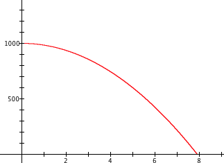
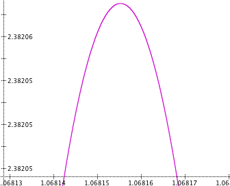
Figure 1.4.1 also illustrates needing to think about behavior over small intervals even when it appears there is nothing unusual about a graph. Looking at variation in x over small intervals reveals "bumpy" behavior we could not see originally in the relationship between x and y.
Figure 1.4.1 At normal scale we see nothing irregular about the graph of $y=x^2+0.0001\sin(10000x)$.
You dealt in prior sections with exceedingly small and exceedingly large quantities. But they were finite nevertheless. You could think of numbers even larger or smaller than the largest or smallest we dealt with and pretend they are measures of something.
In answering Exercise 1.1.2 ("How far away is 1?"), you found that the distance from the 0 to 1 on your screen's y-axis, given the distance from 0 to $10^{-64}$ was about 4 inches, was approximately 1 billion trillion billion trips across the visible universe.
This is an impossibly large physical distance. But we can imagine it and talk about it. Here is a wonderful YouTube video that addresses this very issue—unimaginably large and small numbers in human experience.
In another chapter you will find situations where where you talk about rates of change over "infinitesimally small" intervals, or about the accumulation of variations over intervals having "infinitesimal width".
The phrases "infinitesimally small" and "infinitely large" have been controversial in the history of mathematics. We will not ask you to address that controversy.
Instead, we ask you to form a personal image that, in practice, gives meaning to "infinitesimally small" and "infinitely large" quantities.
We will speak about intervals that are small enough so that, were they any smaller, it would make no essential difference relative to the problem being addressed.
If you must have a definite length to consider as "infinitesimally small", then think of the Planck Length. It is approximately $1.6 \cdot 10^{-35}$ meters. Theoretically, a Planck Length is the smallest length that can be measured.
For practical purposes, you can think of an interval of length one Planck Length on a number line in place of the phrase "infinitesimally small". You can also think of $6.5 \cdot 10^{34}$ meters, the reciprocal of one Planck Length, in place of "infinitely large".
We include this section on zooming in or out on a graph in GC for practical purposes.
A function’s graph sometimes has details that are difficult to see. This is often because the graph’s details are too small or too large to see at the axes’ current scale.
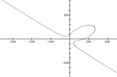
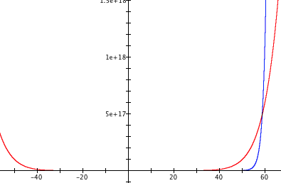
Figure 1.4.1 showed a case where details were too small to see. Figure 1.4.2, below, is a case where details are too large to see. It shows the graph of $y = 2^x$ overlaid with the graph of $y = x^4$.
Many high school textbooks state that exponential growth always overtakes polynomial growth. But in Figure 1.4.2 we see only two intersections, suggesting that $x^4$ is always larger than $2^x$ for values of x larger than some number between 1 and 2.
Therefore, either these textbooks were wrong or there must be some number N so that $2^x\gt x^4$ for all values of $x\gt N$.
In other words, the two graphs must have a third intersection point if exponential growth always outpaces polynomial growth.
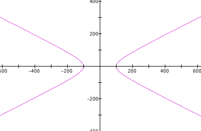
If there is a third intersection point, it is off the screen when the axes are scaled as in Figure 1.4.2. We need to rescale the axes to look for a third intersection of the two graphs.
Figure 1.4.2 suggests that $2^x\gt x^4$ for $x\gt 16$.
When you click on one of GC’s zoom icons, it expands the visible axes (when zooming in) or it contracts the visible axes (when zooming out).
Zooming in is like getting closer to a graph. Your field of vision includes more fine-grained detail in a smaller region of the coordinate plane. Zooming out is like moving away from a graph. Your field of vision includes less fine-grained detail in a larger region of the coordinate plane.
Either way, GC always keeps the origin, or the location of trace crosshairs, in the same place, zooming in or out from it.
You also can rescale vertical and horizontal axes independently. Holding the shift key (command key on Mac) when you click a zoom button re-scales only the vertical axis.
Holding the alt key (option key on Mac) when you click a zoom button re-scales only the horizontal axis.
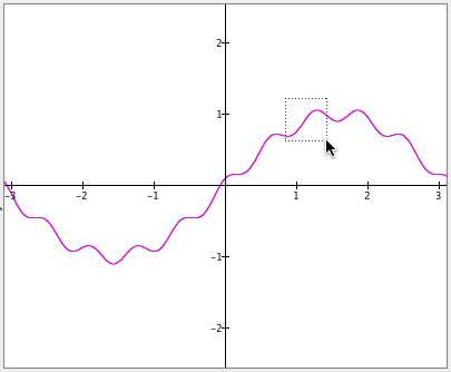
Sometimes you’ll want to zoom in on a section of a graph instead of zooming the entire viewing area. Zoom in a section of a graph by holding the shift key as you click and drag to draw a box around the section you wish to expand.
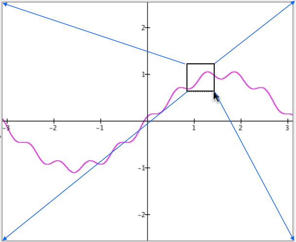
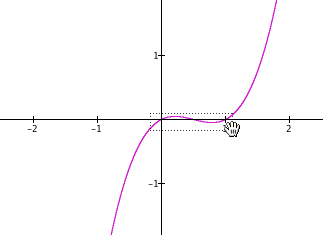
Figure 1.4.3 shows a box being drawn around a section of a graph and what GC does after you release the mouse button.
How you draw a box will determine how you affect the proportions of your zoomed region.
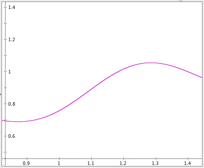
The animation in Figure 1.4.4 shows the sections of a graph being scaled differently according to how the box is drawn. If you want to stretch a section of a graph vertically, draw a short wide box. If you want to compress a section vertically, draw a tall narrow box.
The function’s graph is unaffected. Only the scale of its display is affected.
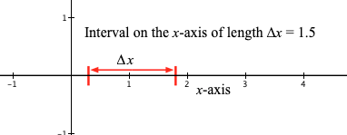
The symbol "$\Delta variable$" (e.g., $\Delta x$) represents the width of an interval through which the variable's value varies. "$\Delta x=1.5$" means an interval of width 1.5 through which the value of x varies. Important: $\Delta x$ represents the width of an interval. It is not the name of an interval.
Exercises 4-7: A section of each displayed graph is boxed. Predict how GC’s display of the graph will appear after releasing the mouse button. Then click the solution link to see how GC actually zoomed that section.
 solution
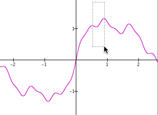 solution
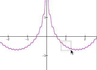 solution
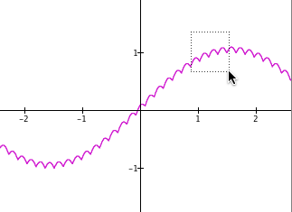 solution
Exercises 8-12: Open each GC file. Click the zoom buttons, with or without modifier keys, to get the view shown for that file.
| < Previous Section | Home | Next Section > |