| < Previous Section | Home | Next Section > |
This ambiguity in uses of "change" can lead to misreading or misinterpreting a statement about "change in x" or "change in y". Does the person or textbook mean change in progress, completed change, or replacing one value by another?
Our uses of "vary", "variation", and "change" is not a rule for you to follow. However, it is important that you be aware of which meaning of "change" you have in mind or someone else intends when using it.
The word "change" in the phrase "rate of change" always has the connotation of change in progress.
The concept of constant rate of change is central to all of calculus. This will become evident in Chapters 4 and 5. In this chapter we will review situations in which the idea of constant rate of change is involved.
In this book we will use a special notation, d[variable], to mean the variable's value varies by small amounts. So, "dx" represents a small variation in the value of x as the value of x varies.
Two quantities vary at a constant rate with respect to each other if all variations in one are proportional to corresponding variations in the other.
If you are told two quantities vary at a constant rate with respect to each other, then you know immediately that all variations in one are proportional to corresponding variations in the other—that $dy=m\cdot dx$ and $dx = \dfrac{1}{m} dy$. The one exception to this is when one quantity has a constant rate of change of 0 with respect to the other. Then the relationship is not reversible.
Let x represent the value of Quantity A and let y represent the value of Quantity B, and let x be the value of Quantity A and y be the value of Quantity B.
Assume that y varies at a constant rate with respect to x. Then, according to the meaning of constant rate of change, any variation in y will be m times as large as the variation in x that corresponds to it for some number m.
We can state the above paragraph symbolically. Suppose that y varies at a constant rate with respect to x. Let $dx$ represents a variation in x. Let $dy$ represents the corresponding variation in y. Then the relationship between variations is $dy=m\cdot dx$ for some number $m$.
If the variation in the value of x is a variation from 0, then $dx=x$ and $dy=m\cdot x$.
The value of y when $x=0$ is represented by the letter b, thus $y=b$ when $x=0$. Therefore, $y=mx+b$ is the general form of the relationship between values of two quantities that vary at a constant rate with respect to each other. The letter m represents the value of that constant rate of change.
Students often wonder why we say that two quantities vary at a constant rate with respect to each other if and only if $dy=m\cdot dx$, that variations in their measures are proportional. They often insist on using the more common definition given below. It turns out that the more common definition is both inaccurate and misleading.
Common, but misleading, definition of constant rate of change:
y varies at a constant rate with respect to x if for a fixed amount of change in x (i.e., $\Delta x$) the amount of change in y (i.e., $\Delta y$) is constant.
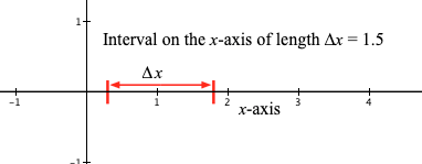
Figure 1.5.0 illustrates why thinking in terms of $\Delta y$ in relation to fixed variations $\Delta x$ is problematic. You must think in terms of variations in y in relation to variations in x within $\Delta x$-intervals, which means attending to $dy$ and $dx$.
Figure 1.5.0. An illustration of why you must think of constant rate of change in terms of relationships between differentials $dy$ and $dx$ instead of relationships between "chunks" of change $\Delta y$ and $\Delta x$.
The top bar in Figure 1.5.1 represents the value of y as the value of x varies. The value of y is b when the value of x is 0. The bottom bar in Figure 3.15.1 represents the value of x. The value of y varies at a constant rate of m with respect to the value of x. As the value of x varies by $dx$, the value of y varies by $m\,dx$. This is true no matter the value of m.
Notice also that the value of $dx$ varies smoothly. Variations are not added wholly. Rather, they vary smoothly. Therefore values of $dy$ vary smoothly so that $dy=m\, dx$ even as $dx$ varies. Move your pointer away from the animation to hide the control bar.
In Figure 1.5.2., the top bar represents the value of y as the value of x varies. The bottom bar represents the value of x. The value of y varies at a constant rate of m with respect to the value of x. The variations in x aggregate to the value of x. The corresponding variations in y aggregate to mx. The value of y is therefore always $y = mx + b$. This is true no matter the value of m.
Reflection 1.5.1. Some people think that Figures 1.5.1 and 1.5.2 say the same thing. Others disagree. Why might each group of people think as they do about Figures 1.5.1 and 1.5.2?
Alert! How you read the next two examples is important. Read them with the goal that you become able to repeat their patterns of reasoning. Do not read them with the goal of remembering what to write!
Stan started running errands in Phoenix at 8:00 am. He had driven 32 km at the end of the last errand. At 11:30 am Stan headed for Tucson at a constant speed of 113 km/hr; 1.6 hours later he began slowing to a stop.
Let D represent the number of km that Stan drove since 8:00 am, and let t represent the number of hours since 8:00 am.
While on his trip to Tucson, the rate of change of D with respect to t was 113 km/hr, so $dD = 113dt$ km, and D, Stan's distance traveled at the constant speed of 113 km/hr, is $D=113(t-3.5)+32$ km.
Why must we subtract 3.5 from t? Because it was not until 11:30 am, when t = 3.5, that Stan began driving at a constant speed.
So it only for $3.5 \le t \le 5.1$ that $D=113(t-3.5)+32$ is a valid model of the distance Stan drove while driving to Tucson. Stan’s distance driven with respect to time did not vary at a constant rate while he ran errands nor after he began slowing down in Tucson.
Reflection 1.5.2. Describe similarities and differences between the story of Stan’s trip and Figures 1.5.1 and 1.5.2.
I am traveling away from home on a straight road at the constant speed of 0.35 km/min. I am 3.8 km from home and I first looked at my watch 7 minutes ago.
Suppose that we are told that Quantity A varied by p kg while Quantity B varied by q liters, $p, q > 0$, and that they varied at a constant rate of m with respect to each other. Let y represent the value of Quantity A and let x represent the value of Quantity B. What is the value of m?
There are two ways to reason about determining the constant rate of change of Quantity A with respect to Quantity B. The first one is to reason quantitatively; the second is to reason algebraically.
Way of Reasoning #1: Look at variations in A relative to a variation of 1 liter in B.
Way of Reasoning #2: Look at total variation in A relative to total variation in B.
The quantitative way of reasoning explains why you compute a constant rate of change by dividing the value of one variation by the value of the other variation.
The algebraic way of reasoning is shorter, but it is about algebra, making it harder to connect with the idea of constant rate of change.
You should strive to think both ways.
Let f be a function having a constant rate of change with respect to its independent variable x. The value of x varies from 7.2 to 9.35.
Let $\Delta x$ represent the variation in the value of x; let $\Delta f(x)$ represent the variation in the value of $f(x)$. Then:
More generally, if the value of x varies from $x=a$ to $x=b$, $a\neq b$ then:
|
Variation in the value of x from $x=a \text{ to } x=b:$ |
$\Delta x=b-a$ |
|
Variation in the value of $f(x)$ from $x=a$ to $x=b:$ |
$\Delta f(x)=f(b)-f(a)$ |
|
Constant rate of change of $f(x)$ with respect to x as the value of x varies from $x=a$ to $x=b:$ |
$\dfrac{\Delta f(x)}{\Delta x} = \dfrac{f(b)-f(a)}{b-a}$ |
The animation in Figure 1.5.3 is similar to that in Figure 1.5.2. It shows an initial value of y (labeled b) and variations in y that are m times as large as variations in x as the value of x varies.
Figure 1.5.3 then shows the upper bar rotating so that it rests upon the end of the bar representing the value of x as it (the value of x) varies.
This is like plotting the value of y above a value of x in a rectangular coordinate system. The result is that the graph of $y=mx+b$ is a line in a rectangular coordinate system.
Use GC for your computations. You might be tempted to use your personal calculator for these exercises. PLEASE DON'T DO THIS. Use GC. It will be by using GC that you will become comfortable using it. Being comfortable with GC will be very important for later chapters.
| < Previous Section | Home | Next Section > |