Ways to Understand Variation, Covariation, and Function
The concept of function began historically, and begins cognitively, with images of quantities whose values vary together (co-variation). Calculus is the mathematics of relationships among quantities whose values vary. So the ideas of covariation and function are foundational to the major concepts and ways of thinking in calculus. (See this article for an analysis of research on covariational reasoning).
The idea of quantity is itself a foundational concept in calculus. However, it is most profitable to understand the meaning of "quantity" in a particular way.
By quantity we shall mean an attribute of an object that you conceive as being measurable.
This means that for you to understand an object's attribute as a quantity, you must understand what it means to measure it. Someone else conceiving an object's attribute as a quantity does not aid your understanding of it.
Example 1: Docking a Boat
This example presents a situation which requests a formula. Our focus will be on on understanding the situation quantitatively so that it is possible to derive a formula.
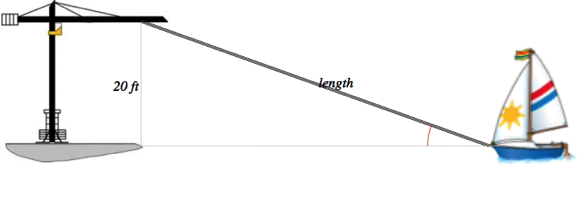
A boat is pulled into a marina by a cable attached to a winch (Figure 3.10.1). A dockhand will take the boat by the bow once it reaches the dock. The winch cable has markings on it so that the winch operator can tell how much cable is out just by looking at the cable.
If the cable's angle from horizontal becomes too great, it will tear the cleat (where the cable attaches) off the boat’s deck. Thus, Bernard, the winch operator, needs to know the angle that the cable makes with the horizontal at each moment that the boat is being towed.
Develop a formula that Bernard can put into his calculator so that he can get the cable’s angle from horizontal simply by entering the cable's length into this formula.
Figure 3.10.1 A boat being towed into a dock by a cable from a winch.
The first thing to notice about Figure 3.10.1 is that, in the figure, nothing varies. You must envision the figure so that things in it vary according to the description of the situation.
Think about what varies and what stays the same in Figure 3.10.1 before playing the animation in Figure 3.10.2.
Figure 3.10.2. Some quantities's values vary and some quantities' values are constant. Some quantities' values are irrelevant to the question.
Quantities in the towed boat scenario
We can conceive many quantities in this scenario. Some will have values that are constant; some will have values that vary. Some will be relevant to the question; some will be irrelevant to the question.
The winch's weight. Varies as cable is pulled in; not relevant to the question.
The boat's height. Constant as cable is pulled in; not relevant to the question.
Winch's height from the dock. Constant as cable is pulled in; perhaps relevant to the question.
Boat's distance from the dock. Varies as cable is pulled in; perhaps relevant to the question.
Length of cable from winch to boat. Varies as cable is pulled in; definitely relevant to the question.
Measure of cable's angle from horizontal. Varies as cable is pulled in; definitely relevant to the question
Independent quantity: Length of cable from winch to boat. The cable's length varies.
Dependent quantity: Measure of cable's angle from horizontal. The measure of the cable's angle from horizontal varies as the cable's length from winch to boat varies.
The measure of the cable's angle from horizontal varies as the length of cable varies. We say that the angle's measure is a function of the cable's length because each cable length determines exactly one angle measure.
If we let $\theta$ represent the measure of the cable's angle from horizontal and let L represent the cable's length, then $\sin(\theta)=20/L$, so $\theta=\mathrm{arcsine}(20/L)$. The value of $\theta$ varies as the value of L (the cable's length) varies.
The function arcsine is the inverse of sine. If $-\pi/2 \le u \le \pi/2$ and $\sin(u)=v$, then $v=\mathrm{arcsine}(u)$. To graph the relationship between cable length and angle in GC, type $$y=\asin(20/x),\, x>20$$ where x represents the length of cable between winch and boat, y represents the angle's measure, and "asin" is GC's word for "arcsine".
Reflection 3.10.1. We said, "The measure of the cable's angle from horizontal is a function of the length of cable between winch and boat because each cable length determines exactly one angle measure."
Could we have said, "The cable's length from winch to boat is a function of the measure of the cable's angle from horizontal because each angle measure determines exactly one cable length"?
If so, would this have helped to answer the question?
Example 2: Distance between clock hands
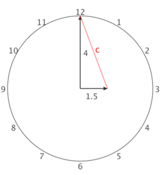
A clock keeps time from 3:00 to 7:00. The hour hand is 1.5 inches long; the minute hand is 4 inches long (Figure 3.10.3). What is the distance between clock hands' tips as elapsed time varies?
Figure 3.10.3. Distance between tips of clock hands as elapsed time varies from 3:00 to 7:00.
The first thing to notice about Figure 3.10.3 is that, in the figure, nothing varies. You must envision the figure so that things in it vary according to the description of the situation.
Think about what varies and what stays the same in Figure 3.10.3 before playing the animation in Figure 3.10.4.
Figure 3.10.4. Some quantities's values vary and some quantities' values are constant. Some quantities' values are irrelevant to the question.
Quantities in the clock scenario
We can conceive many quantities in this scenario. Some will have values that are constant; some will have values that vary. Some will be relevant to the question; some will be irrelevant to the question.
The clock's diameter at each moment of elapsed time. Constant as elapsed time varies; not relevant to the question.
Length of minute hand at each moment of elapsed time. Constant as elapsed time varies; perhaps relevant to the question.
Length of hour hand at each moment of elapsed time. Constant as elapsed time varies; perhaps relevant to the question.
Elapsed time (number of hours since 3:00). Varies as time passes; definitely relevant to question.
Measure of angle made by minute hand and horizontal at each moment of elapsed time. Varies with elapsed time; perhaps relevant to question.
Measure of angle made by hour hand and horizontal at each moment of elapsed time. Varies with elapsed time; perhaps relevant to question.
Angular rate at which minute hand revolves at each moment of elapsed time. Constant as elapsed time varies ($2\pi$ radians per hour); not relevant to the question.
Angular rate at which hour hand revolves at each moment of elapsed time. Constant as elapsed time varies ($2\pi/12$ radians per hour); not relevant to the question.
Measure of angle between minute hand and hour hand (angle with horizontal of minute hand minus angle with horizontal of hour hand) at each moment of elapsed time. Varies with elapsed time; definitely relevant to the question
Distance between tips of minute and hour hands at each moment of elapsed time. Varies with elapsed time; definitely relevant to the question.
Independent quantity: Number of hours elapsed since 3:00. Elapsed time varies.
Dependent quantity: Distance between tips of minute and hour hands at each moment of elapsed time. Varies with elapsed time.
Notice that we listed the rates at which hour and minute hands revolve with respect to elapsed time as quantities in the situation. They were not relevant to the question of distance between tips at each moment in time. However, had the question been, "At what rate is the distance between hour and minute hands' tips varying with respect to time?", these quantities would definitely have been relevant to the question.
The distance between tips of minute and hour hands varies as number of hours since 3:00 varies. We say that the this distance is a function of elapsed time because each number of hours elapsed determines exactly one distance between tips of minute and hour hands..
If we let $\theta_1$ represent the measure of the minute hand's angle with horizontal at each moment of elapsed time, and let $\theta_2$ represent the measure of the hour hand's angle with horizontal at each moment of elapsed time, then $\theta=\theta_1-\theta_2$ represents the measure, from minute hand to hour hand, of the angle they form at each moment of elapsed time.
With these relationships among quantities we can use the Law of Cosines to represent the distance between the hands' tips at each moment of elapsed time (i.e., at each number of hours since 3:00).
Reflection 3.10.2. Let $\theta_1$ be the measure of the angle made by the minute hand and horizontal at each moment of elapsed time. Is $\theta_1$ a function of elapsed time? Could we say the same about the hour hand? Explain.
Example 3: Homer's distances from Springfield and Shelbyville
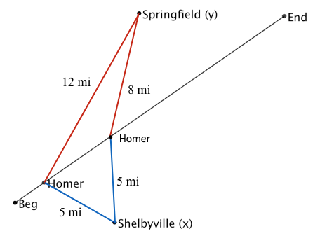
Homer Simpson drives on a segment of road that is north of Shelbyville and south of Springfield (Figure 3.10.5). Is his distance from Shelbyville a function of his distance from Springfield? That is, does each distance from Shelbyville determine a unique distance from Springfield?
Figure 3.10.5. Homer's distances from Springfield and Shelbyville as he drives along a road.
Quantities in the Homer scenario
We can conceive many quantities in this scenario. Some will have values that are constant; some will have values that vary. Some will be relevant to the question; some will be irrelevant to the question.
The length of the road segment that Homer drives. Constant; not relevant to the question.
Homer's distance from the beginning of the road segment. Varies; perhaps relevant to the question.
Homer's distance from Shelbyville at each of Homer's distances from the beginning. Varies with Homer's position on the road.
Homer's distance from Springfield at each of Homer's distances from the beginning. Varies with Homer's position on the road.
Independent quantity: Homer's distance from Shelbyville at each of Homer's distances from the beginning. Varies with Homer's position on the road.
Dependent quantity: Homer's distance from Springfield at each of Homer's distances from the beginning. Varies with Homer's position on the road..
For Homer's distance from Springfield to be a function of his distance from Shelbyville, each Homer-Shelbyville distance must be associated with exactly one Homer-Springfield distance.
Figure 3.10.6 shows that this is not the case. Homer can be 5 miles from Shelbyville at two locations on the road. So Homer's distance from Springfield when he is 5 miles from Shelbyville could be 12 miles or 8 miles. This violates the condition that a relationship between quantities must satisfy for one to be a function of the other.
Figure 3.10.6. Homer can be at two different distances from Springfield while he is at one distance from Shelbyville. Distance from Springfield is therefore not a function of distance from Shelbyville.
Homer's distance from Springfield is not a function of his distance from Shelbyville. If someone tells you, "Homer is 5 miles from Shelbyville", you cannot be certain whether he is 12 miles from Springfield or 5 miles from Springfield.
The boxed comment above conveys the purpose of the idea of a function in mathematics. If someone tells you that y is a function of x, then you can be certain that, once they provide the rule of association between y and x, you can determine a value of y uniquely (i.e., with certainty) whenever you are given a value of x.
Example 4. Behavior of functions defined by a rule of association
Examples 1, 2, and 3 presented scenarios involving relationships among quantities defined contextually. The contexts theselves provided the information necessary to understand the relationships and to decide whether the relationships defined one quantity as a function of another.
Functions defined contextually might seem less mathematical than functions defined by a formula. However, as we saw in Examples 1 and 2, defining a function contextually in terms of quantities and relationships was necessary to define it by a formula.
In some cases, we will study the behavior of quantities whose function relationship is defined by a mathematical formula to begin with. We can use the same ways of thinking as we did with related quantities in contextual relationships in these more abstract instances in order to understand how the value of y varies as the value of x varies.
Consider the relationship $y=x^2-x$.
We know that
$x^2-x=0$ when $x=0$ and $x=1$
$x^2\lt x$ when $0\lt x\lt 1$
$x^2\gt x$ otherwise
As the value of x varies from 0 in either direction, $x^2$ increases slowly at first and increases more rapidly as x varies.
From these observations we can get a general sense of the covariation between values of y and values of x.
Let the value of x start at 0 and become more negative.
$y=x^2-x$ starts at 0.
As the value of x becomes more negative, $x^2\gt x$, so the value of y increases.
The more negative x becomes, the faster the value of y increases.
Let the value of x start at 0 and increase to 1.
$y=x^2-x$ begins at 0 and ends at 0
As x moves from 0 to small positive numbers, $x^2$ becomes less than x, so y decreases to slightly negative values.
As x continues to increase to 1, the value of $x^2$ is still less than x but they become closer together until $x=1$ where the value of y is again 0.
Let the value of x continue increasing from 1.
$y=x^2-x$ begins at 0.
As the value of x increases from 1 to become more positive, the value of $x^2$ becomes greater than x, so the value of y increases.
The more positive x becomes, the faster the value of y increases
Putting these observations together, we can generate a graph of corresponding values of x and y, as seen in Figure 3.10.7
Figure 3.10.7 An animation to illustrate the reasoning in Example 4.
Exercise Set 3.10.1
Each of (a)-(c) describes a scenario involving many quantities. In each case,
List each quantity
State whether it varies or is constant
State whether it is relevant to the question
State independent and dependent quantities
Explain whether one quantity is a function of the other.
A rubber ball is shot vertically from an air gun at a height of 10 meters. The ball's initial vertical velocity is 15 meters/sec. Acceleraton from gravity is -9.8 meters/sec. After how many seconds does the ball hit the ground?
Water is pumped into an empty spherical water tank of radius 5 meters at the rate of 450 liters/min. What is the water's height in the tank after x minutes?
A truck driver earns $\$18$/hour. Maintenance to operate the truck costs $\$0.73$/mi. Fuel is $\$3.05$/gal. Fuel mileage is 9 mi/gal at 40 mi/hr and decreases 0.6 mi/gal per increase of 10 mi/hr. What is the total cost to drive the truck M miles at S mi/hr, $S\ge 40$?
Analyze the behavior of y with respect to x in the same way as Example 4.
$y=\sqrt{x}+0.1\sin(10x),\,x\ge 0$
Keep in mind that $-1\le \sin(u)\le 1$.
$y=x^3-x^2+x$
Think about ways different terms dominate over different intervals.
$y=x\sin(x)$
Homer Simpson's Distances from Springfield and Shelbyville
We concluded in Example 3 that distance from Springfield is not a function of distance from Shelbyville. But there is still a relationship between them in that each has a value at each of Homer's distances from the road's beginning.
The animation below depicts Homer Simpson driving his car along a straight road from its beginning to its end. It also shows Homer's distance from Shelbyville on the horizontal axis and his distance from Springfield on the vertical axes.
Your task is to
Keep track of Homer's distance from Springfield in relation to his distance from Shelbyville as he drives along the road.
Sketch a graph of that relationship in the coordinate system shown to the right (you will need to draw your own axes).
Imagine a correspondence point in your coordinate system for the two distances, then keep track of it by imagining it sprinkled with Pixie dust. The Pixie dust will leave a trace of everywhere the correspondence point has been.
Make a concerted effort to do this before clicking on the solution link.
The animation below shows Homer driving along the same road as in Exercise 3.10.5 except that he occasionally backs up. How will this affect the graph of Homer's distance from Springfield in relation to his distance from Shelbyville? Explain.
Download this file. You can move the locations of Springfield and Shelbyville by clicking and dragging. Move Shelbyville, Springfield, or both so that distance from Springfield is a function of distance from Shelbyville. Print your file. Write an explanation of why this relationship is now a function.
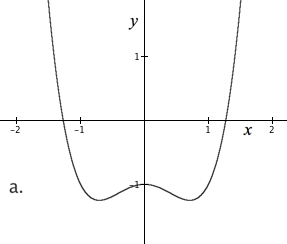
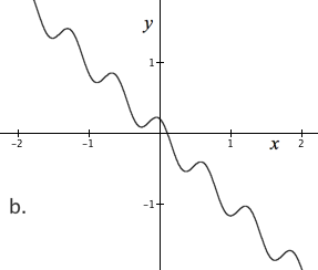
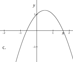
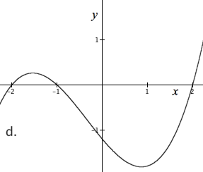
Graphs (a)-(d) are displayed below. In each case, analyze the behavior of y in relation to x. Define y as a function of x to generate a graph that is in principle the same as the one displayed.
You will need to reverse the style of thinking presented in Example 4.
Functions Defined Implicitly
The fundamental idea of a function is that values of variables are related in such a way that knowing the value of one variable allows you to determine exactly one value of the other. Though today’s formal definition of a function evolved over the past several centuries, the basic idea never changed — a function is a relationship between variables that has the property that each value of one variable determines exactly one value of the other.
For several centuries, mathematicians used equations to represent relationships between variables.
For example, in the equation $x+2y=4$, as soon as we know a value of y, the value of x is determined uniquely (there is only one value of x that is determined by a given value of y).
Similarly, as soon as you know a value of x in the equation $x+2y=4$, the value of y is determined uniquely.
If you consider x the independent variable in $x+2y=4$, then y is a function of x.
If you consider y the independent variable in $x+2y=4$, then x is a function of y.
When you write an equation to represent a functional relationship between two variables, and either of them can be taken as independent, you must state which of them you are taking as independent.
Not all equations provide a choice of which variable can be taken as independent when representing a functional relationship between them. If you want $x+y^2=4$, where x and y are real numbers, to represent a functional relationship, then you have no choice which variable to take as independent.
If you take x to be independent, then when $x=0$, $y=2$ or $y=-2$. This means that there is some value of x for which a value of y is not determined uniquely. On the other hand, no matter the value we assign to y, the value of x is determined uniquely. Therefore in the equation $x+y^2=4$, x is a function of y but y is not a function of x.
If, however, we restrict values of y in $x+y^2=4$ to $y\ge 0$, then each value of x less than or equal to 4 determines a value of y uniquely. Therefore, in $x+y^2=4$, where $x\le 4$ and $y\ge 0$, either x or y could be taken as independent and $x+y^2=4$ would represent a functional relationship between x and y.
Today, we distinguish between two ways of representing a relationship between variables. We represent a relationship explicitly by writing the dependent variable to the left of the equal sign and on the right side writing a description of how to determine the dependent variable’s value from a value of the independent variable.
We represent a relationship implicitly by representing the relationship in a way that we must give additional information about which variable to take as independent.
The equation $x+y^2=4$, with y the independent variable, represents a relationship between values of x and values of y implicitly. The same relationship between x and y is represented explicitly by the equation $x=4‑y^2$. We do not need to state which variable is independent when we represent a relationship between variables explicitly. It is good practice in both cases to state the domain of values that the independent variable can have. In this book we use the custom that an independent variable’s value can be any real number unless stated otherwise, or unless the context makes the restriction clear.
Whether we represent a relationship between variables explicitly or implicitly, for a relationship between variables to be called a function, each value of the independent variable must determine exactly one value of the dependent variable.
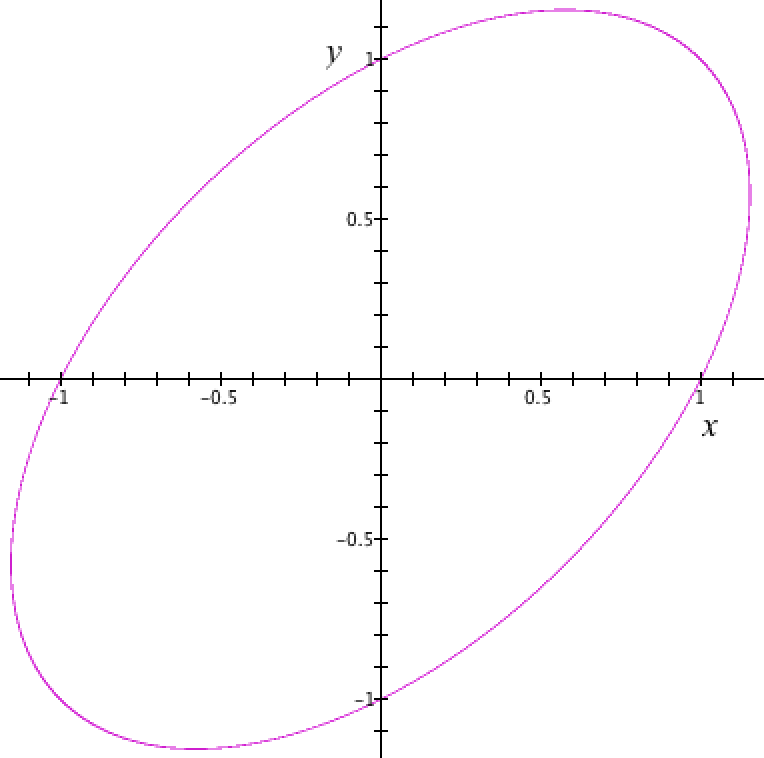
Recall that the graph of a mathematical statement involving two variables is the set of ordered pairs whose coordinates make the statement true. Figure 3.10.8 displays the graph of $x^2-xy+y^2=1$ in rectangular coordinates. That is, Figure 3.10.8 displays the set of points {(x, y)}, where x and y are real numbers such that $x^2-xy+y^2=1$}.
Figure 3.10.8. The displayed graph of $x^2-xy +
y^2=1$.
It is clear from the displayed graph of $x^2-xy+y^2=1$ that values of x are not determined uniquely from values of y when 0 ≤ y ≤ 1. We can show this by displaying the graph of y = 1 on top of the graph of $x^2-xy+y^2=1$, 0 ≤ y ≤ 1 (Figure 3.10.9). Figure 3.10.9 shows that the value $y=1$ determines two values of x, namely $x=0$ and $x=1$. When animated, Figure 3.10.9 also shows that each value of y, $0\le y\le 1$, determines two values of x.
Figure 3.10.9. Each value of y, $0\le y \le 1$, determines two values of x.
You can show symbolically that $y=1$ determines two values of x in $x^2-xy+y^2=1$. Substitute 1 for y in $x^2-xy+y^2=1$, getting $x^2-1x+12=1$. The solutions of the equation $x^2-x+1=1$ are $x=0$ and $x=1$. Therefore $y=1$ determines two values of x.
What restrictions could we put on values of x so that values of x are determined uniquely by values of y between 0 and 1? Clearly, the restriction $-1 ≤ x ≤ 0$ when $0\le y\le 1$ works. Thus, $x^2-xy+y^2=1$ represents x as a function of y when y is taken as the independent variable, $-1\le x\le 0$, and $0\le y\le 1$.
An examination of Figure 3.10.8 suggests that, with a suitable restriction on values of x, there are values of y smaller than 0 and values of y larger than 1 for which we can determine x as a function of y. We can determine the appropriate values by finding values of y in $x^2-xy+y^2=1$ that give exactly one value of x, by finding values of x that give exactly one value of y, and then use those values to restrict y and x.
If we think of y as a parameter in $x^2-xy+y^2=1$ instead of as a variable, then we can use the quadratic formula to find values of y that give just one value of x, as shown in Figure 3.10.10.
Figure 3.10.10. The quadratic formula applied to
$x^2-xy+y^2=1$ by thinking of y as a
parameter.
We are looking for values of y that are solutions to $$(-y)^2-4(y^2-1)=0,$$ because when the determinant in Figure 3.10.10 is 0, each of those values of y will determine exactly one value of x. We also want values of x that determine exactly one value of y. Solving for y in $$(‑y)^2-4(y^2-1)=0$$ gives us $y=\pm \sqrt{\frac{4}{3}}$. Substituting $\sqrt{\frac{4}{3}}$ for y in $$x^2-xy+y^2=1$$ gives $x=\pm 0.5 \sqrt{\frac {4}{3}}$. Similarly, solving for x in $$(‑x)^2-4(x^2-1)=0$$ gives $x=\pm \sqrt{\frac{4}{3}}$ and $y=\pm0.5 \sqrt{\frac {4}{3}}$.
By examining Figure 3.10.8 we can tell which values of x go with which values of y. We want $$-0.5 \sqrt{\frac {4}{3}} \le y \le \sqrt{\frac {4}{3}}$$ and $$-\sqrt{\frac {4}{3}} \le x \le 0.5\sqrt{\frac {4}{3}}.$$
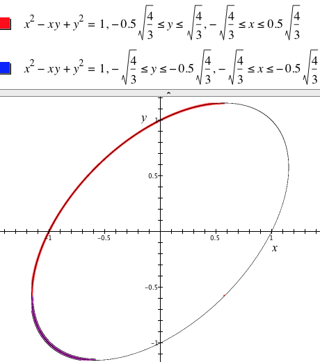
Therefore, $$x^2-xy+y^2=1, -0.5 \sqrt{\frac {4}{3}} \le y \le \sqrt{\frac {4}{3}}, -\sqrt{\frac {4}{3}} \le x \le 0.5\sqrt{\frac {4}{3}}$$ represents x as a function of y (see the portion of Figure 3.10.11’s graph in
red).
But we could include more of the ellipse than the part highlighted in red and still have x as a function of y. We could also include the section of the ellipse in
blue (Figure 3.10.11). Figure 3.10.11 shows the restrictions on x and y that generates the blue section of the ellipse.
Figure 3.10.11. The highlighted section of the displayed graph of $x^2-xy+y^2=1$ represents x as a function of y.
Even though we have two sets of restrictions on x and y in Figure 3.10.11, the restrictions together are such that each value of y in its domain (namely, $-\sqrt{\frac {4}{3}} \le y \le \sqrt{\frac {4}{3}}$ is related to exactly one value of x. Therefore, with these restrictions on x and y, $x^2-xy+y^2=1$ represents x as a function of y.
Exercise Set 3.10.2
Use GC to display a graph of $3x^2-2y^2=4$. Restrict the domain of x and the domain of y in two different ways so that the displayed graph shows x as a function of y over the largest possible domains of x and y. You might have to do this in two parts.
Use GC to display a graph of $3x^2-2y^2=4$. Restrict the domain of x and the domain of y in four different ways so that the displayed graph shows y as a function of x over the largest possible domains of x and y. You might have to do this in two parts.
Express y as a function of x explicitly for each of the following equations. Include restrictions on the domains of x and y so that they are as large as possible. Use GC to check your answers.
$3x^2-2y^2=4$
$x^3-y^3=3$
$3x-2y=7$
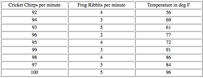
One summer Raul visited a lake on several different evenings and took data regarding temperature, frogs and crickets. At the end of the summer, he organized his data into the following table.
Make two scatter plots, one for number of chirps per minute and temperature, and one for number of ribbits per minute and temperature. Make temperature the dependent variable (vertical axes) for each.
Is temperature a function of the number of chirps per minute according to the entries in this table? Explain why or why not. Is temperature a function of the number of ribbits per minute according to the entries in table? Explain why or why not.
Consider the number of cricket chirps per minute in relation to the number of frog ribbits per minute.
Is the number of cricket chirps per minute a function of the number of frog ribbits per minute? Explain.
Is the number of frog ribbits per minute a function of the number of cricket chirps per minute? Explain.
This temperature exercise gives a clue as to why the term 'function' was chosen as the name for mathematical functions.
Here is how the word 'function' is defined outside of mathematics. Use this temperature context to describe how the meaning of 'function' outside of mathematics relates closely to the definition of function in mathematics. Talk about both chirps and ribbits in your answer.