| < Previous Section | Home | Next Section > |
| Rectangular Coordinates | Polar Coordinates | Mixed-Scale Coordinates | Two Perspectives | Exercises |
A two-dimensional coordinate system is a method for locating points in the plane. It is also a method for representing the values of two quantities simultaneously. It was by Descartes’ ingenious method of representing the location of points in a plane or in space that we can visually represent relationships between quantities’ values.
The Cartesian, or rectangular, coordinate system locates points by representing quantities’ values separately on two number lines that are perpendicular to each other, and then combining them to locate a point in the plane whose location represents the quantities’ values simultaneously.
Example:
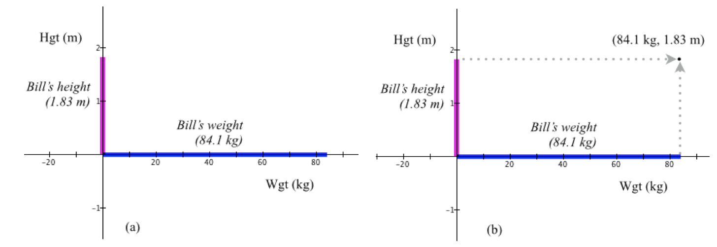
Every person has a height and has a weight (mass). Suppose we want to represent individuals’ heights and weights simultaneously. Figure 3.8a shows Bill’s weight (84.1 kg) on the horizontal axis and his height (1.83 m) on the vertical axis. Figure 3.9.1a represents Bill’s height and weight, but separately.
Figure 3.9.1 (a) Bill’s height, in meters is represented on the horizontal axis. Bill’s weight, in kg, is represented by the segment on the vertical axis. (b) The correspondence between Bill’s height and weight is represented by the location of the point having coordinates (84.1, 1.83).
Figure 3.9.1b combines the two separate representations into one representation—the point whose location is 84.1 units from the vertical axis and 1.83 units from the horizontal axis.
The point with coordinates (84.1, 1.83) is called the correspondence point for these particular values of Bill’s weight and height. It is a point that represents Bill’s weight and height simultaneously.
More generally, a correspondence point is made by taking the values that co-occur in the quantities you are relating as coordinates of a point in your coordinate system. A correspondence point’s location in any coordinate system represents values of two (or more) quantities simultaneously.
If we could record Bill’s height and weight continuously, we would have a record of of every correspondence point between his height and weight. Figure 3.9.2 is a hypothetical graph of Bill height (in meters) in relation to his weight (in kg) recorded continuously over his first 20 years. Each point on this graph represents Bill’s height when he was a particular weight.
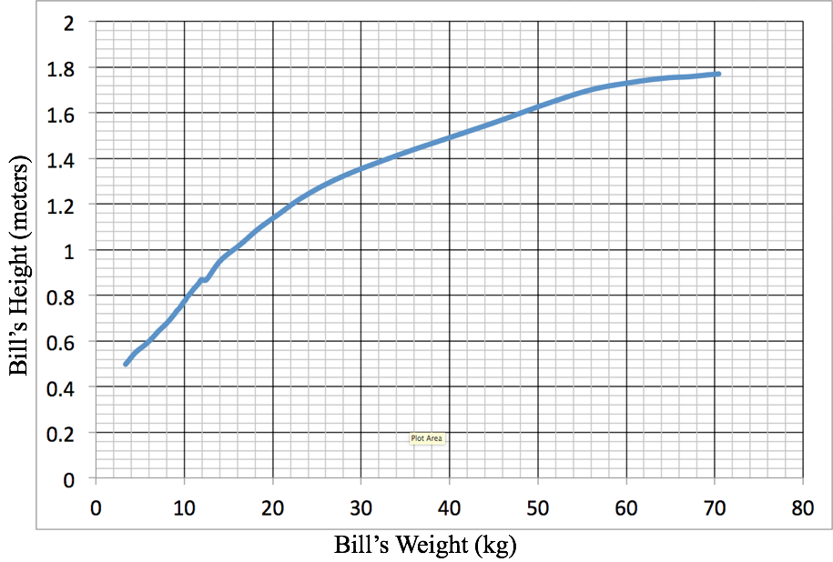
Reflection 3.9.1. The point with coordinates (10.55 0.80) is on the graph in Figure 3.9.2. What does the location of this point represent about Bill’s weight and height?
Reflection 3.9.2. What is your best estimate of Bill’s birth height and birth weight? What assumption must you make?
Reflection 3.9.3. Why does the displayed graph in Figure 3.9.2 start at (3, 0.5) instead of starting at (0,0)?
Reflection 3.9.4. Bill claimed that his weight and height stayed at 25.68 kg and 1.28 m for two years. Is his claim inconsistent with the graph in in Figure 3.9.2? Explain.
Reflection 3.9.5. The displayed graph of Bill’s height in relation to his weight is not realistic in several ways. Describe one way in which it is not realistic.
Sometimes you will identify a variable in a mathematical statement as the variable that is under your control, in the sense that you may choose values for it. Variables whose values you consider under your control are called independent variables.
A dependent variable is a variable whose value becomes determined once you assign a value to an independent variable. It is customary in a rectangular coordinate system to put values of an independent variable on the horizontal axis and values of a dependent variable on the vertical axis. But this is just a custom. It is not necessary. However, if you break custom, you should state which variable you are taking as independent and which you are taking as dependent.
In some situations, variables will be neither dependent nor independent. The situation in Figure 3.9.2 is an example. Bill’s weight does not depend on his height, nor does Bill’s height depend on his weight. The graph in Figure 3.9.2 simply keeps track of them together. You could put either quantity on either axis.
A rectangular coordinate systems is like a street map of Phoenix (an exceptionally flat city). Locations are determined by intersections of lines that are perpendicular to axes.
A polar system works like radar. A point’s location is recorded according to its distance from a reference point and its angle from a reference direction.
The reference point is called the system’s pole and the ray from the pole in the reference direction is called the polar axis.
Figure 3.9.3 illustrates the polar coordinate system. Angles are measured in radians (see the Sections 2.2, 2.3, and 2.4). Distances from the pole are measured in units of the radius of the unit circle. Coordinates in the polar plane are customarily in the form $(r,\theta)$, where r is the point’s distance from the pole and θ is the measure in radians of the angle formed by a ray from the pole to the point and the reference direction.
A point with coordinates (3, 1.2) in the polar system is 3 unit lengths from the pole in a direction of 1.2 radians from the polar axis.
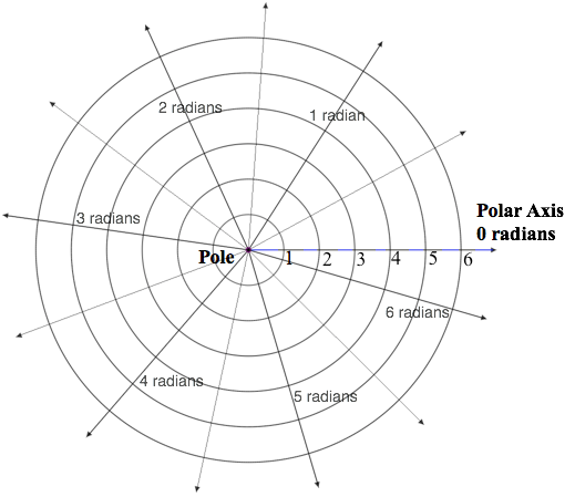
Figure 3.9.3 The polar coordinate system. Rays point in directions,
measured in radians from the polar axis. Circles designate distances
from the pole, measured in units of the radius of the unit circle.
Coordinates of a point are given as (distance from pole, direction from
polar axis).
The animation in Figure 3.9.4 shows a way to think of determining a point’s location in the polar plane. First determine its distance from the pole, then determine the direction from the polar axis.
Figure 3.9.4. Locate a point in the polar coordinate system by first determining its distance from the pole and then determining its direction from the polar axis.
Many people find the convention for ordered pairs in polar coordinates unnatural. The first coordinate is r, but it is easier to think first of a point’s direction.
Imagine a ray pointing in the direction of $\theta$, then imagine going r units in that direction (backing up if r is negative).
Thinking of a point’s direction first also fits with the fact that $\theta$ often is taken as the independent variable when displaying a graph in polar coordinates.
You are free to think of locating a point by any method you find most natural. Just remember that the order of the coordinates is $(r,\theta)$ when you represent a point in the polar plane.
Points in the polar plane do not have unique coordinates. Figure 3.9.5 shows a point in the polar plane located in two ways, both in the form (r, θ). The point in Figure 3.9.5 can be located by the pair $(3.7 \text{ miles}, 0.69 \text{ radians})$ and it can be located by the pair $(‑3.7 \text{ miles}, 0.69\, - \pi \text{ radians})$ where $0.69 - \pi\text{ radians}=-2.45\text{ radians}$.


Figure 3.9.5. Points in the polar plane do not have unique coordinates. The point in this figure has coordinates $(3.7, 0.69)$ or $(-3.7, -2.45)$
To imagine a graph in the polar plane, imagine varying the independent variable a little at a time while simultaneously keeping track of the dependent variable’s value. Record the covariation using the conventions of your coordinate system. In most situations in which we use polar coordinates, we will treat θ as the independent variable and r as the dependent variable.
Imagine two quantities whose values are represented by r and $\theta$, and that they have the relationship that $r=2\theta - 5$. To represent this relationship in the polar plane, vary the value of $\theta$, keeping track of its value and the value of r.
Recall that in the polar plane, $\theta$ is a number of radians measured from the reference direction and r is a number of unit lengths from the pole in the direction of θ. Figure 3.9.6 shows points with coordinates $(r,\theta)$ where $r=2\theta - 5$. Be sure that you understand what the coordinates of each ordered pair represent and why these points are located where they are.
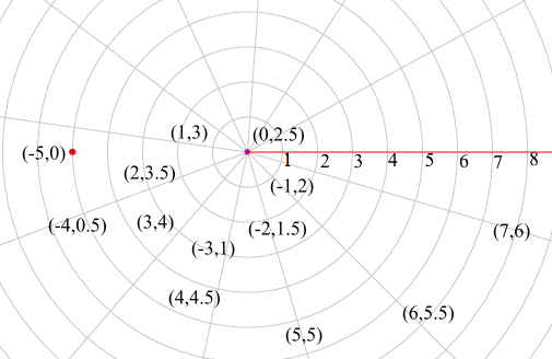
Figure 3.9.6. Points for r = 2θ - 5 plotted in the polar plane. They appear jumbled, making it hard to see a pattern in their generation.
It is quite hard to envision the complete graph of r = 2θ - 5 in polar coordinates just from plotted points. The plotted points are too jumbled to convey what happens as θ varies. A complete graph of f in polar coordinates for 0 ≤ θ < 2π is given in Figure 3.9.7.
Imagine a ray, originating from the pole, being swept counter-clockwise as θ varies from 0 to 2π radians. At the same time that you sweep a ray from 0 to 2π radians, imagine the location at a distance of 2θ – 5 units in the direction that the ray points—going forward when 2θ – 5 is positive, and backward when 2θ – 5 is negative.
Figure 3.9.7. Graph of $r=2\theta-5$ as $\theta$ varies from 0 to $2\pi$.
Statisticians and scientists are fundamentally interested in relationships between statistical variables. In exploratory data analysis they often graph data within different coordinate systems in order to judge visually whether a relationship is linear, quadratic, cubic, or exponential (among others).
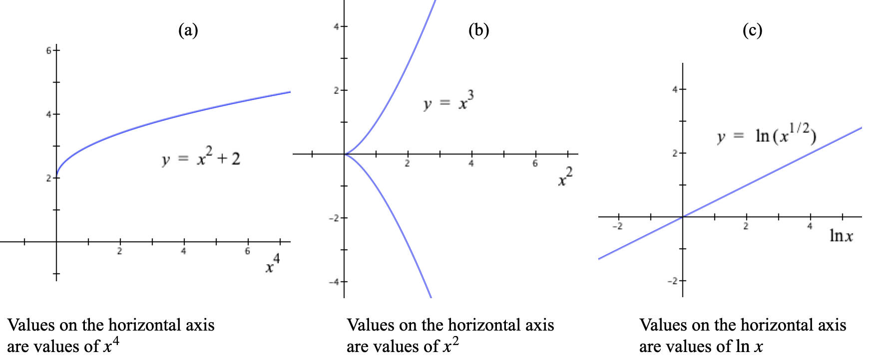
Their method is to use coordinate systems with the vertical axis scaled so that plotted data appears to lie on a line if variables are related in specific ways. Such coordinate systems are called mixed-scale coordinate systems. Figure 3.9.8 illustrates three common mixed-scale systems:
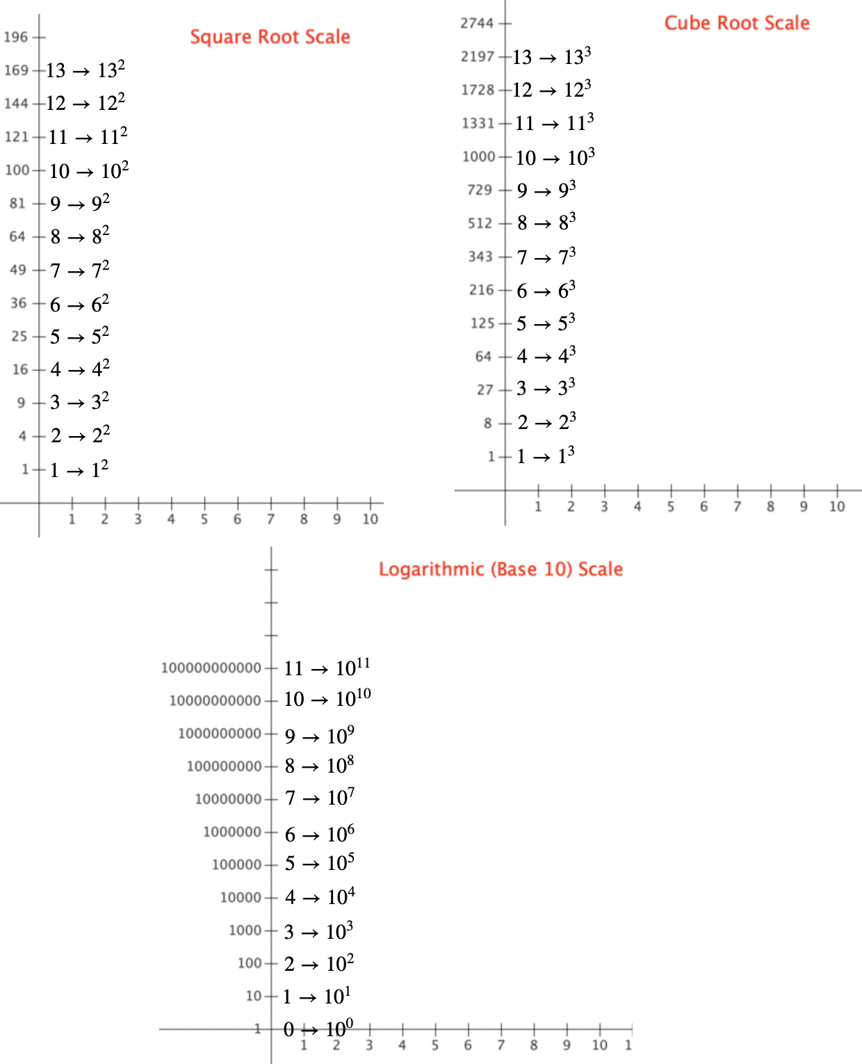
Figure 3.9.8. Three coordinate systems with different scales on the y-axis. The arrow ($\rightarrow$) means "stands for".
Read, for example, "$11\rightarrow 10^{11}$" as "11 units from 0 stands for a y-value of $10^{11}$".
The names of the scales might seem backward—that "Square root scale" should be "Quadratic scale" and "Logarithmic scale" should be "Exponential scale". The names of the scales actually reflect what you do to the y-value of a data pair to plot it in one of these coordinate systems.
Figure 3.9.9 illustrates the same set of data plotted in Quadratic, Cubic, and Logarithmic scales.
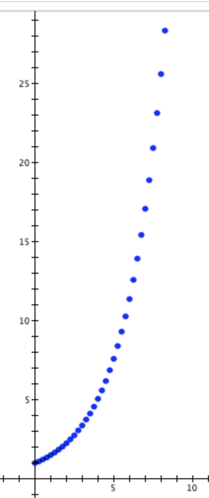
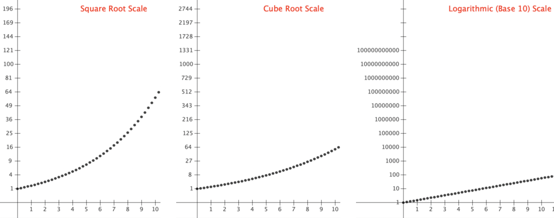
Figure 3.8.9. One data set (on top) plotted with three diferent y scales.
The third graph shows data points from the original graph falling along a line when plotted using the Logarithmic scale. This means $y=a\cdot 10^bx$ for some numbers a and b. This is because, in the logarithmic scale, we plotted $(x,\log(y))$. If $y=a\cdot 10^{bx}$, then $$\begin{align} \log(y)&=\log(a\cdot 10^{bx})\\[1ex] &=\log(a)+\log(10^{bx})\\[1ex] &=\log(a)+bx\log(10)\\[1ex] &=\log(a)+bx\cdot 1\\[1ex] &=\log(a)+bx \end{align}$$
Notice that the right side is a linear function in x. The scaled values of y in each data point $(x,y)$ end up plotted along a line with equation $\log(y)= \log(a)+bx$.
A question sometimes arises as to which comes first, a point or its coordinates. The answer is, "It depends on the context."
Sketch a graph that displays a record of the value of u in relation to the value of v.
Imagine a correspondence point, then keep track of it by imagining it sprinkled with Pixie dust. The Pixie dust will leave a trace of everywhere the correspondence point has been.
a) ( click for solution)
b) ( click for solution)
c) ( click for solution)
d) ( click for solution)
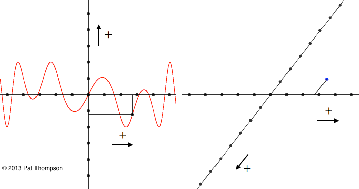
The arrows in each system indicate the positive direction for each axis.
The highlighted point in the left system is plotted in the right system.
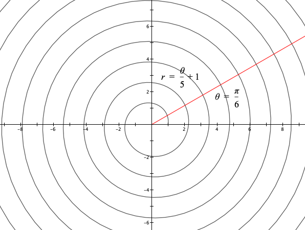
Sketch the displayed graph on the left within the coordinate system on the right. Do the two displayed graphs represent the same relationship?
 ( solution)
Remember that polar coordinates are in the form $(r,\theta)$.
How far apart are two successive points that lie on the same ray from the pole? (Graphs of $r=m\theta$, m a non-zero real number, are called Archimedean Spirals)
What are the coordinates of the point on the graph that is at the pole? Why does the graph never pass through (0, 0) even though it passes through the pole?
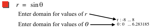
Why does this graph make a circle? What is its center and radius?
This graph is called the Batman Curve. Explain how the variation in $\theta$ relative to r over the following intervals produces a piece of the displayed graph (It might help to print a graph of y = sin(x) in Cartesian coordinates.): $$\begin{align} -&8\le r\le -7\\[1ex] -&7\le r\le -6\\[1ex] -&6 \le r\le -5\\[1ex] &5\le r\le 6\\[1ex] &6\le r\le 7\\[1ex] &7\le r\le 8\\[1ex] \end{align}$$
What does this tell you about a point on the graph of $y=\cos(x)$?
What does it tell you about a point on the graph of $r=\cos(\theta)$?
The displayed graphs are different. Are the graphs themselves different? Explain.
Recall the meaning of a statement’s graph from Section 3.5. Also recall that coordinate pairs in rectangular coordinates are in the order (value of independent variable, value of dependent variable), regardless of how you label your axes..
| < Previous Section | Home | Next Section > |