| < Previous Section | Home | Next Section > |
When you write on paper with a pen, you leave behind specks of ink. The writing appears solid to the eye because the specks are close together.
So it is with computer images. Images (such as the letters in this sentence) appearing on a computer screen are a collection of square dots.
These dots are called pixels. Computer screens commonly have over 80 pixels per cm, and smart phones screens commonly have over of 128 pixels per cm. Pixels on computer screens have become so small that most images appear to the eye as smooth.
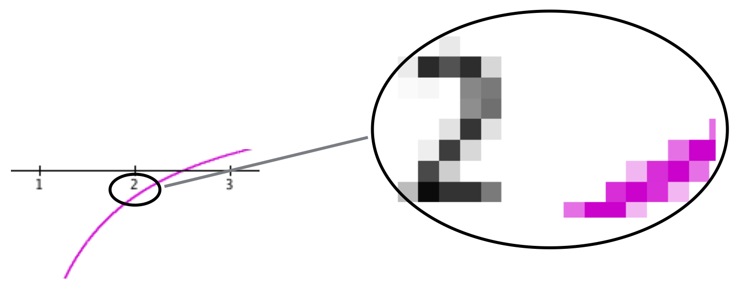
However, if you were to magnify an image on the screen so that you also magnify the pixels that make it, you would see that what appears smooth to the eye is not really smooth. It is jagged.
Figure 3.6.1 shows a small piece of a graph plotted on a computer screen in Cartesian coordinates and an enlarged image of the same piece. The enlargement shows the highlighted screen pixels that make up the original portion of the plotted graph.
Figure 3.6.1. Images on a computer screen are made of highlighted pixels.
Many people imagine that graphing programs match statements typed into them with a library of shapes. This way of thinking could not be farther from the way computers actually draw graphs.
Here is a way to envision how GC generates a mathematical statement’s graph. Imagine that you have just typed a statement like y = some expression in x, and then pressed Enter. Here is a way to imagine what GC does to generate its displayed graph:
When you press Enter, GC goes through all the steps listed above, but very quickly—so quickly that the graph seems to appear instantaneously.
From this moment on, strive to imagine that GC varies the independent variable’s value rapidly and smoothly on its visible axis, from smallest value to largest, one pixel at a time. One way to do this is, for any statement, mentally scan along the independent variable’s axis, imagining the graph being created as you scan.
Even more importantly, imagine that GC varies the value of the independent value smoothly within pixels to judge what shading it should give the plotted point. GC’s method of creating a graph by varying the value of the independent variable is illustrated in Figure 3.6.2.
Figure 3.6.2. As the value of x varies smoothly, GC plots the
points (x, y) where y = ecos x.
Move your cursor away from the animation to make the control bar disappear.
A keyboard shortcut is a letter or combination of letters and modifiers that tell GC to do the same thing as a menu selection. For example, ctrl-Enter is a keyboard shortcut for the menu selection Math/New Expression. Click here for a brief list, or here for a full list, of GC shortcuts for Mac. Click here for a brief list, or here for a full list, of GC shortcuts for Windows.
It is convenient to see the coordinates of specific points on a GC graph. Click on a point to see it’s coordinates. Drag to move the cross hairs along the graph, as in Figure 3.6.3. Clicking and dragging on a GC-displayed graph is called tracing the graph. Move your cursor away from the animation to make the control bar disappear.
Figure 3.6.3. Click on a point; GC displays its coordinates. Drag sideways after clicking to select other points. The crosshairs "snap" to zeroes and extrema as you drag the pointer.
For parts b, c, d, and e, explain the statement’s graph’s behavior: Why does it increase where it increases? Why does it decrease where it decreases? Why does it increase or decrease more or less rapidly over some intervals than others?
a) 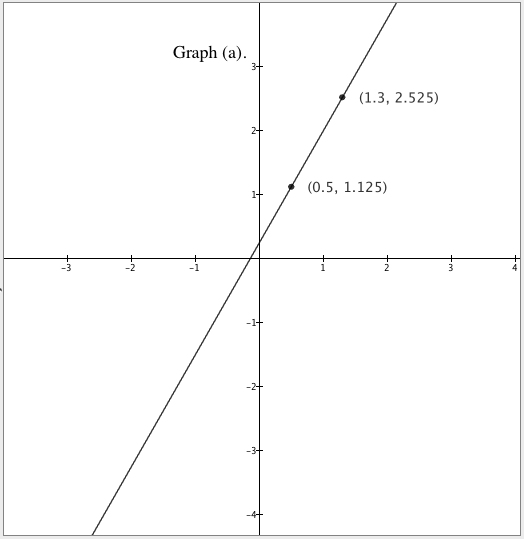
b) 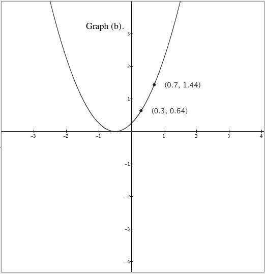
c) 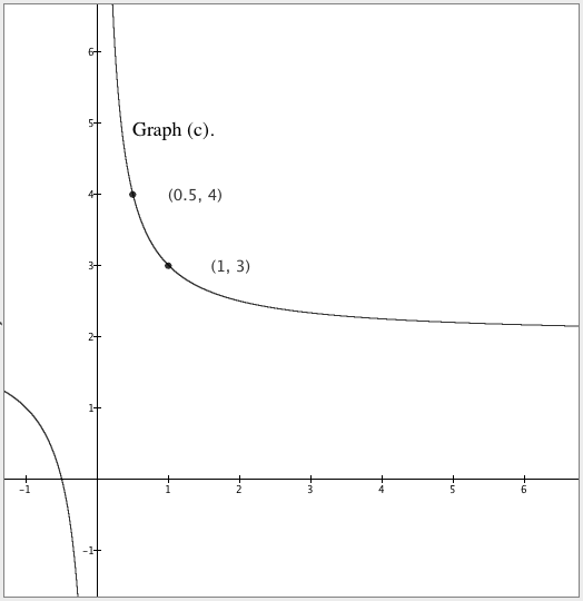
d) 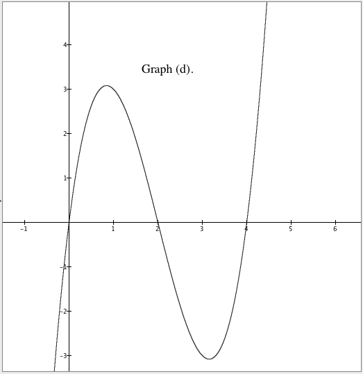
e) 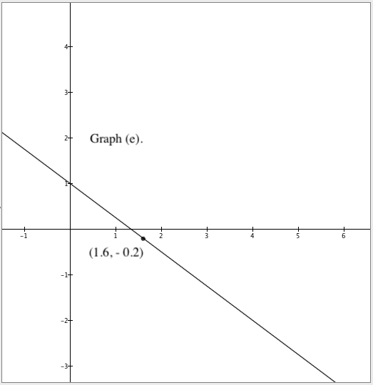
f) 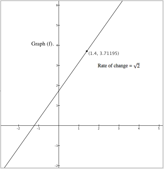
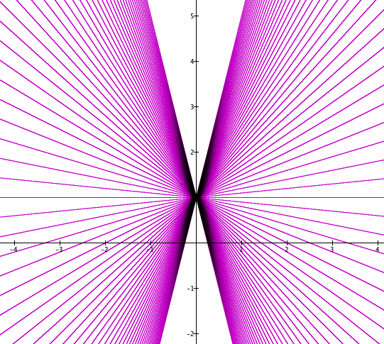
Here is a family of graphs defined by $y=mx+1\text{, } m \in \{-4.0, -3.9, -3.8, ..., 3.8, 3.9, 4.0\}$. Use the meanings of variable, parameter, and constant to explain how GC made this image. You will need to talk about how GC displays graphs.
| < Previous Section | Home | Next Section > |