| < Previous Section | Home | Next Section > |
A graph is not a picture. Rather, a graph is a set of ordered pairs of numbers. When you plot a graph’s ordered pairs in a coordinate system, according to the conventions of that system, you get a visual representation of the graph. The representation of a graph you see results from merging the conventions of the coordinate system with the set of ordered pairs being plotted. The graph of y = 2x + 1 is the set of ordered pairs (x,y) such that x and y are real numbers, and y = 2 x + 1. The pairs (0.1, 1.2), (0.4, 1.8), (2.7, 6.4) are all in the graph of y = 2x + 1.
In general, the graph of a mathematical statement involving two variables (such as) u and v is the set of ordered pairs $$\{(u,v) \text{ such that the values of }u \text{ and } v\text{ make the statement true}\}.$$
A mathematical statement's displayed graph is the statement's graph displayed within the conventions of a coordinate system. Even though people shouldn't, they often use the terms graph and displayed graph interchangeably. Just keep in mind that a graph's displayed appearance depends upon the conventions of the coordinate system in which it is displayed.
A convention (or custom) is a way of doing something or writing something, among many possibile alternatives, that a community agrees upon to aid communication. Mathematics is rife with conventions. But they are not rules. They are agreed-upon ways of doing something.
It is customary that the first coordinate in a pair is a value of the relationship's independent variable and the second coordinate is a value of the relationship's dependent variable. But this is only customary.
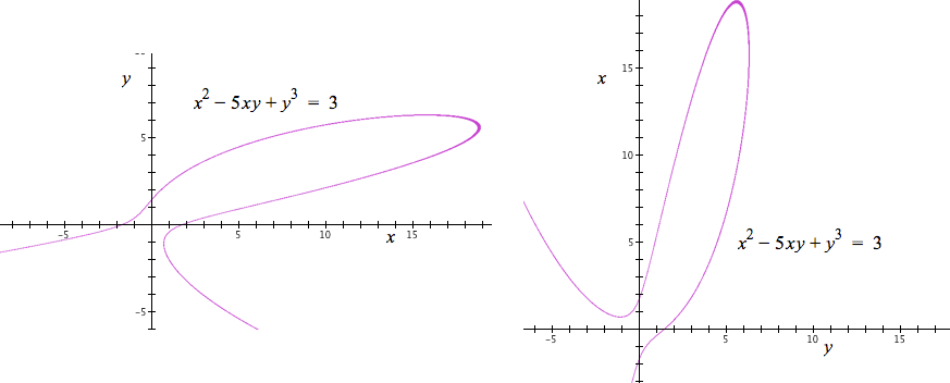
Also, a mathematical statement might not have an independent or dependent variable. The equation $x^2-5xy+y^3=3$ (see Figure 3.5.1, left) does not have an independent or dependent variable. You can also depart from conventions in displaying its graph (see Figure 3.5.1, right).
In Figure 3.5.1 (right), the graph of $x^2-5xy+y^3=3$ is displayed within a rectangular coordinate system, but values of x are located on the vertical axis and values of y are located on the horizontal axis.
Figure 3.5.1. Graph of $x^2-5xy+y^3$ displayed in Cartesian (rectangular) coordinates in two ways. Neither x nor y can be taken as an independent variable, and values of x and y are placed on axes according to two different conventions.
Figure 3.5.2 shows the graph of $v=2u+1$ displayed in two different coordinate systems. On the left, the graph of $v = 2u + 1$ appears as a line in a rectangular (Cartesian) coordinate system because it is conventional in rectangular coordinates that values of the independent variable (in this case u) are located on the horizontal axis and values of the dependent variable (in this case v) are located on the vertical axis.
Figure 3.5.2 (right) shows the graph of $v=2u+1$ in a polar coordinate system. It appears as a spiral because, in polar coordinates, values of v give the radius of a circle centered at the pole and values of u give a direction from the pole. The graph (set of ordered pairs) is the same in both cases, but in different coordinate systems the graph of $v=2u+1$ appears differently.

Figure 3.5.2. Two displays of the graph of $v=2u+1$. Left: Displayed in a rectangular coordinate system. Right: Displayed in a polar coordinate system. The same graph (set of ordered pairs) appears differently in different coordinate systems.
As we explain more fully in Section 3.9, the coordinates of a point $(u,v)$ when displayed in Cartesian coordinates are read from left-to-right.
In the polar system, due to Isaac Newton, coordinates in the polar system are written $(r,\theta)$, where the value of r (typically, the dependent variable) is the radius of a circle centered at the pole and the value of $\theta$ (typically, the independent variable) is a direction from the pole.
Points displayed in polar coordinates therefore seem to have their coordinates reversed from Cartesian conventions.
Of course, you can depart from any convention in a coordinate system as long as you state clearly how you departed from it.
Figure 3.5.3 shows an image commonly found in calculus textbooks. It is usually offered as depicting a change in x in relation to a change in y. But many students have difficulty seeing anything in the graph varying.
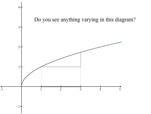
Figure 3.5.3.
Figure 3.5.4 offers a way to view a static graph to envision variables varying within it.
Figure 3.5.4. Static graphs depict relationships dynamically when you envision values of variables varying.
It is up to you to inject dynamic relationships into static graphs. You will see variation all the time with practice making the effort to see it.
| < Previous Section | Home | Next Section > |