Section 4.9
Exact Rate of Change Functions

Here are three scenarios where all we know about a quantity is its rate of change at a moment. We do not know how much of the quantity there is.

Scenario I

Companies with fleets of drivers often keep records of each driver’s speed (in km/h) at successive moments of elapsed time during the day. But they do not record the number of km that the car has traveled at any moment during the day.

Let r be the function that gives a drivers speed (rate of change of distance traveled with respect to time) at each moment in time during the day. Anyone looking at these records would know the the value of $r(t)$, the rate at which a driver’s distance varied with respect to time, at values of t.

Let d be the function that relates a driver’s distance traveled that day since the day began and let t represent the number of hours since the work day began. Then a value of $r(t)$ gives the rate of change of the driver’s distance traveled that day (in km/h) at the moment that t hours has elapsed in the work day.

Question: Could we reconstruct the driver’s number of km traveled from the beginning of the day up to any moment in time during that day just by knowing the car's speed at each moment during that day and the number of hours that have elapsed up to that moment?

Scenario II

Objects near Earth’s surface accelerate due to gravity at -9.8 $\frac{m/s}{s}$, meaning that its velocity (in m/s) varies at a constant rate of -9.8 m/s every second. This number ignores air resistance (addressed in a later chapter).

Gravitational acceleration being -9.8$\frac{m/s}{s}$ means that while an object falls after being released, its upward velocity increases -9.8 m/s every second. So its velocity will be $v(t) = -9.8t$ m/s, where t is the number of seconds since being released.

Let $d(t)$ be the distance that the object has fallen in t seconds after it was released. Then each value of $v(t)$ gives the rate of change of d with respect to time at the moment it has fallen t seconds.

That is, after an object is released we can know its rate of change of distance with respect to time at any moment during its fall, but we do not know how far it has fallen up to that moment.

Question: Could we determine how much the object’s distance from its release point has varied at every moment during its fall just by knowing its acceleration due to gravity and the number of seconds that it has fallen up to that moment?

Scenario III

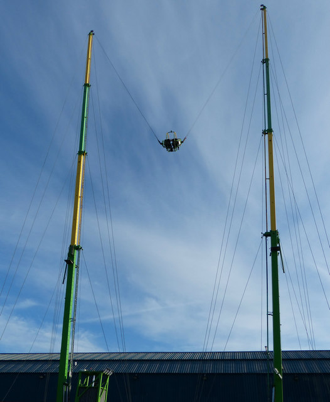
Let w be a function that gives the mechanical work accomplished at a moment in time during one cycle of pulling an amusement park’s slingshot sling backward before it is released (Figure 4.9.1).

We are given that each value of the function $r_w(t) = 500\cos(\frac{t}{5}), 0 ≤ t ≤ 15.7$ sec, gives the momentary rate of change with respect to time of $w(t)$ in Newton-meter/sec.

Question: Could we determine how much the applied mechanical work varied from the beginning of a cycle up to any moment within that cycle just by knowing how fast this work varied with respect to time at each moment and the number of seconds that have elapsed up to that moment?

Common Theme Across Scenarios

In each of the three scenarios, we knew the rate at which one quantity varied with respect another at every moment of the independent variable. We did not know how much there is of either quantity.

The question in each scenario is whether it is possible to recover the variation in a quantity up to a particular moment of its independent variable just by knowing its rate of change at every moment of its independent variable.

As we explain in Chapter 5, the answer, in principle, is "yes".

The functions in Scenarios I-III give the rate of change of another function at every moment of their independent variables. They are called exact rate of change functions. Every value of an exact rate of change function gives the rate of change at a moment for another function.

In preparation for Chapter 5, we will take a closer look at what it means that one function gives the rate of change of another function at every moment of the other function’s independent variable.

The Meaning of "Essentially Equal To …"

It is common in mathematics to represent the exact value of a number when in actuality we cannot produce the number's exact value. Examples include $\sqrt 2$, $\pi$, and e. You can enter the symbols $\pi, e,\text{ or}, \sqrt 2$ into a calculator and it will produce a number, but the number it produces is an approximation to the actual value.

Food for thought: If we can produce no better than an approximation to a number, what, then, could we mean by the number's "actual value"?

As of March 2019, the best approximation to the value of π has 31 trillion digits. Even then, this is still an approximation. How do we know this 31 trillion digit number is a "good" approximation of π? Because someone proved that given any level of tolerance, you can repeatedly apply the method they used so that, at some point, all further approximations will be closer together than this level of tolerance.

The idea of essentially equal is based on having a method that produces approximations to a conceptually-defined number that you can argue become indistinguishable from each other at any level of tolerance. When you reach a point where you get no better approximations at your current level of tolerance (e.g., $1/1,000,000$), you can say your approximation is essentially equal to this conceptually-defined number.

The Babylonians had a method for approximating square roots. It looks like this in the case of $\sqrt 2$:

$$\begin{align} x_0&=1\\[1ex] x_1&=(x_0+2/x_0)/2\qquad (1.5)\\[1ex] x_2&=(x_1+2/x_1)/2\qquad (1.41667)\\[1ex] x_3&=(x_2+2/x_2)/2\qquad (1.41422)\\[1ex] x_4&=(x_3+2/x_3)/2\qquad (1.41421- \text{correct to 6 significant digits}) \end{align}$$

If we set a tolerance of 1/100,000, then any approximation after $x_4$ will be indistinguishable (at this level) from 1.41421. You can see a GC implementation of this recursive method by clicking here.

In other words, the method $x_{n+1}=(x_n+2/x_n)/2$ eventually produces values indistinguishable from each other at any tolerance level we set. When values approximating $\sqrt 2$ become indistinguishable from each other at our chosen level of tolerance, we have a value essentially equal to the number we represent symbolically as $\sqrt 2$.

By "$f(x)$ is essentially equal to $g(x)$ at a moment of x", we mean for any tolerance we set, there is an interval $(a,b)$ with $a\lt x\lt b$ such that for all values of x in the interval the difference between values of $f(x)$ and values of $g(x)$ are within that tolerance.

Put more plainly, for any tolerance we set, we can zoom in around the point $(x,f(x))$ so that the two graphs are indistinguishable by the criterion we set.

When we say that $r_f(x_0)$ is the momentary (exact) rate of change of f at $x_0$, we mean that the values of $f(x_0+dx)$ are essentially equal to the values of $f(x_0)+r_f(x_0)dx$ as $dx$ varies through a sufficiently small interval containing $x_0$.

We cannot allow dx to be 0. This is because we want to say that $dy/dx$, the quotient of the differential in y and the associated differential in x, gives us the same information as $dy=m\cdot dx$. If we allow dx to be 0, then $dy/dx$ is meaningless.

We shall use the symbol "$\doteq$" to represent the relation "essentially equal to". Thus, we would write $1.999...\doteq 2$ to mean "terms in the sequence 1.999... become indistinguishable from 2".

We can therefore use "$\doteq$" to say the following about approximating variations in $f(x)$ near a value $f(x_0)$:

Suppose values of $r_f(x)$ give the momentary rate of change of $f(x)$ for all values of x. Then, for any value $x_0$ of x, and for sufficiently small variations dx from $x_0$, $$f(x_0+dx)\doteq f(x_0)+r_f(x_0)dx.$$

The Meaning of a Value of an Exact Rate of Change Function

The function $r_f$ is an exact rate of change function for the function f when every value $r_f(x)$ gives f's momentary rate of change for that value of x.

Scenario III included a definition of the function $r_w$ as $r_w(t) = 500\cos(\frac{t}{5}), 0 \le t \le 15.7$ sec. Read "$r_w(t)$" as "r sub w of t", which is short for "the momentary rate of change (r) of (the function) w at a value of t".

The conceptual definition of $r_w$ was that each value $r_w(t)$ for a specific value of t gives the momentary rate of change of the amount of mechanical work accomplished in pulling the sling backward before releasing it. What does that mean?

First, remind yourself of what it means that a function has a rate of change at a moment $x_0$. It means that the function has a rate of change that is essentially constant over an interval containing $x_0$.

Suppose that $t = 1.25$. Then $r_w(1.25) = 500\cos(\frac{1.25}{5})$, or $r_w(1.25) = 484.456$ Newton-meters/sec.

Since any value of $r_w(t)$ is w’s rate of change at at the moment of a value of t, we are assured that for some interval containing $t = 1.25$, w varies at a rate that is essentially constant, and in this instance that rate of change is 484.456 Newton-meters/sec.

At this rate of change, if dt, the variation in t, were to vary from 0 to 0.0001, then dw, the variation in the value of w, would vary from 0 to $484.456\dot 0.0001$ Newton-meters.

Put another way, evn though we do not know the value of $w(1.25)$, we do know that $w(1.25+0.0001)-w(1.25)$, the actual variation in w, is approximately equal to $484.456\cdot 0.0001$ Newton-meters. So, if 0.0001 is a sufficiently small variation in t, then $$\begin{align} w(1.25+0.0001)-w(1.25)&\doteq r(1.25)\cdot 0.0001,\qquad \text{or}\\[1ex] w(1.25+0.0001)&\doteq w(1.25) + r(1.25)\cdot 0.0001 \end{align}$$ after t has varied from $t=1.25$ to $t=1.2501$.

In the previous sentence we were required say "the actual variation in w, $w(1.25 + 0.0001) ‑ w(1.25)$ is essentially equal to $r(1.25)\cdot(0.0001)$ Newton-meters".

This is because we are only assured that the rate of change of w with respect to t is essentially constant over some interval of time from $t = 1.25$ to $t = 1.25+dt$ seconds, and this interval might be smaller than 0.0001 seconds.

We can nevertheless say that if w were to vary at a constant rate of $r(1.25)$ Newton-meters/sec over the time period $t = 1.25$ to $t = 1.2501$ seconds, then the value of w would increase (essentially) by $dy=r(1.25)dt$ Newton-meters, where $0\lt dt\le 0.0001$.

Symbolically, $w(1.25+dt)\doteq w(1.25)+r(1.25)dt$.

In Section 4.4 (Rate of Change at a Moment) we emphasized that a function f having a rate of change at a moment $x_0$ meant that f’s rate of change over some interval containing $x_0$ is essentially constant, and hence f’s graph over that interval, in Cartesian coordinates, would be essentially linear.

In the present situation, since w has $r_w(1.25)$ as its rate of change at the moment that $t = 1.25$, the graph of w would be essentially linear over sufficiently small intervals around $t = 1.25$.

But the graph of w being linear over an interval means that the graph of $y = r_w(x)$ would be essentially constant over that same interval. So we can think of the graph of w being made of short, essentially straight line segments, and the graph of $r_w$ as being made of short, essentially flat line segments.

Figure 4.9.2 gives a visual illustration of the ways that all these meanings interact.

• The value of $r(1.25)$ is the momentary rate of change of w with respect to x at the moment that $x = 1.25$.
• The function w having a "rate of change at the moment $x=1.25$" means that w has a rate of change that is essentially constant over some interval containing $x = 1.25$. This means that the function r, being the rate of change function for w, is essentially constant with a value of $r(1.25)$ over that interval.
• The left graph shows the graph of r as having essentially the constant value of $r(1.25)$ as x varies from 1.25 to 1.2501.
• The right graph assumes, for purposes of illustration, that $w(1.25) = 10.1$.
• As dx varies from 0 to 0.0001 the value of x varies from 1.25 to 1.2501. The essential (approximate) value of w varies at the constant rate of $r(1.25)$. Therefore the value of $w(1.25+dx)$ as dx varies from 0 to 0.0001 is essentially $w(1.25) + dy$, or $w(1.25) + r(1.25)dx$.

It will be beneficial to remind yourself of what w, r, 0.0001, dx, and dy represent about the scenario in which they occurred.

• The value $w(x)$ gives the mechanical work accomplished up to the moment of x seconds in one cycle of drawing the slingshot.
• The value $r_w(x)$ gives the rate at which work varies with respect to time at the moment that x seconds have elapsed from the beginning of a cycle.
• The value 1.25 seconds was one moment during the cycle.
• The value 0.0001 seconds was the width of the interval we decided was sufficient for $r(1.25)$ to be essentially constant.
• dx was the variation in x as x varied through the interval from $x = 1.25$ to $x = 1.2501$. In other words, as the value of dx varied from 0 to 0.0001, $x = 1.25 + dx$
• dy was the variation in w as dx varied from 0 to 0.0001.

It is important to notice something that can easily become lost. Because we know w’s rate of change at each moment we have a good idea of how much $w(x)$ varies over every interval of sufficiently small width--despite not knowing anything about values of w or its definition. In Chapter 5, we will use this important insight to re-create a function by knowing only its rate of change function.

We can generalize Figure 4.9.2 in several ways.

• Our assumption that $w(1.25) = 10.1$ was arbitrary. We assumed it simply so that we could start w’s graph somewhere. But the variation in w would be essentially equal to $r_w(1.25)\cdot(0.0001)$ regardless of the actual value of $w(1.25)$.
• We could have picked an arbitrary value for x, such as $x = x_0$. The momentary rate of change of w with respect to x at $x = x_0$ would be $ r_w(x_0)$.
• We could have picked an interval with a width other than 0.0001, such as a width of ∆x. So, as dx varies through the interval from 0 to ∆x, $x = x_0 + dx$ for all values of dx.
• Our reasoning would have been the same. We would end with $w(x_0+dx)\doteq w(x_0)+r_w(x_0)dx$ for $0 \lt dx \le \Delta x$.

Figure 4.9.3. gives another illustration of a value $r_f(c)$ being the exact rate of change of a function f at the moment $x=c$. It gives an exact rate of change function for a function f where $r_f(2)=0.834$. The animation shows this means $f(2+dx)\doteq f(2)+dy$, over a suitably small interval, where $dy=0.834 dx$.

Figure 4.9.3. What it means that a function has a rate of change at the moment that $x=2$.

Exercise Set 4.9

1. Values of the function f give the volume of concrete being added to a floor of a New York skyscraper during a 45-second pour. Values of the function $r_f$ defined as $r_f(x) = 2e^{-x/15}$ give the rate of change of f in $\mathrm{m^3/sec}$ at each moment of x, $0\le x\le 45$ seconds.
1. Examine the graph of $y = r_f(x), 0 ≤ x ≤ 45$ in GC. Use the graph to describe the flow of concrete during a 45-second pour.
   Type "r ctrl-L f → ctrl-9 x = …" to define $r_f$ in GC. Type $y = r_f(x), 0 ≤ x ≤ 45$ to generate the graph. Scale the horizontal axis to see the entire graph.
2. At what rate is concrete being poured at the moment that 5.2 seconds has elapsed during the pour?
3. At 5.2 seconds of pouring, 8.79 $\mathrm{m}^3$ of concrete had been poured. Approximately how much concrete will have been poured at 5.4 seconds of pouring? Explain your work.
4. Approximately how much concrete will be poured between 5.2 and 6 seconds? Use one variation of 0.8 seconds.
5. Revise your estimate in part d by estimating how much concrete is poured every 0.2 seconds from 5.2 seconds to 6 seconds. Why are the estimates different? Hint: Examine the graph of $y = r_f(x)$.
6. You were told in part c that $f(5.2) = 8.79 \mathrm{m}^3$. Use your work in part e to sketch a graph by hand of $y=f(x), 5.2\le x\le 6$. Scale your axes conveniently.
2. Values of the function $r_g$ defined as $r_g (x) = 100 - x^2$ give the rate of change of a function g at each moment of x, $0 ≤ x ≤ 10$.
1. Examine the graph of $y = r_g (x), 0 ≤ x ≤ 10$ in GC. Use the graph to describe behavior of g over that interval.
   Type "r ctrl-L g → ctrl-9 x = …" to define $r_g$. in GC. Type $y = r_g (x), 0 ≤ x ≤ 10$ to generate the graph. Scale the vertical axis to see the entire graph.
2. What is g’s rate of change when $x = 4.5$? What does this number mean?
3. $g(4.5) = 419.625$. Approximately how much will the value of g vary as the value of x varies from $x = 4.5$ to $x = 4.6$?
4. Approximately how much will the value of g vary as the value of x varies from $x = 4.5$ to $x = 5.5$? Use one variation of 1 second.
5. Revise your estimate in part d by estimating how much g will vary from $ x = 4.5$ to $x = 4.6$, from $x = 4.6$ to $x = 4.7$, $\cdots$, from $x = 5.4$ to $x = 5.5$. Why are the estimates different? Hint: Examine the graph of $y = r_g (x)$.
6. You were told in part c that $g(4.5) = 419.625$. Use your work in part e to sketch a graph by hand of $y = g(x), 4.5 ≤ x ≤ 5.5$. Scale your axes conveniently.
3. Define h in GC as $h(t) = 4\cos(2t)$. Graph $y = h(x)$.
1. Define a linear function f whose graph passes through the points $(3.01, h(3.01))$ and $(3.02, h(3.02))$. Graph $y = f(x)$.
   
   The graph of $y = f(x)$ should appear to be tangent to the graph of h at $x = 3.01$. Why?
2. Revise your definition of f so it passes through the points $(n, h(n))$ and $(n + 0.01, h(n + 0.01))$. Graph $y = f(x)$.
   
   Click on "n" in the n-slider. Change n's lower bound to -3 and upper bound to 3. Click OK, then click n’s play button. What happens? Why?
3. What do Parts (a) and (b) have to do with differentials and rates of change at a moment?