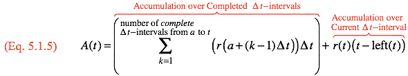
Equation 5.1.5. The approximate accumulation function in one line.
| < Previous Section | Home | Next Section > |
In Chapter 4, Section 4.9 we developed the idea that knowing a function’s rate of change at a moment of its independent variable gives information about how much the function varies during that moment:
We do not know f's value at any moment, but we have a good approximation of how much it varies during any moment. We will return to this idea repeatedly.
The concept of an accumulation function is quite general.
When the measure of Quantity A varies at some rate of change with respect to the measure of Quantity B, Quantity A accumulates variations at a rate that is essentially constant in relation to sufficiently small variations in B. From Chapter 4, this is the meaning of Quantity A having a rate of change at a moment of Quantity B.
Defining a function whose values give the net accumulation of one quantity by knowing its rate of change at every moment of its accumulation addresses the first foundational problem of calculus. Namely,
When we know a function’s rate of change at every moment of its independent variable, we can estimate the function’s net variation as its independent variable varies. We do this by accumulating variations in the function’s value as they occur while the value of its independent variable passes through successive moments.
An accumulation function is a function that is generated by accumulating variations in its value. The variations occur at some rate over moments of its independent variable.
In the remainder of this chapter we will
Reminder to Windows users: You cannot type "$\Delta x$", "$\Delta t$" etc. in GC. Instead, type "\Dx\", "\Dt\", etc. Windows gives no easy way to type the character "∆".
Reminder to Mac users: To type "$\Delta x$", "$\Delta t$" etc. in GC, type "\option-j x\", "\option-j t\", etc. The keystroke option-j gives the character "$\Delta$" on a Mac.
A team of enginering students designed a rocket-powered basketball for their course project.
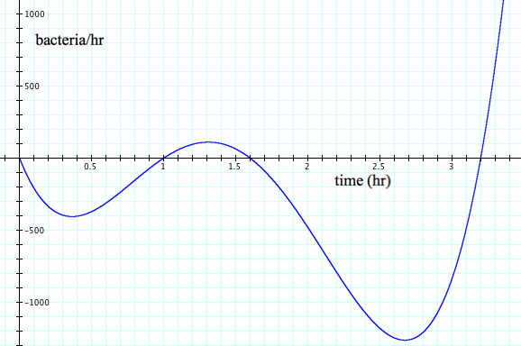
They designed the motor so that within the first 90 seconds after launch, the rocket will have a rate of change of height with respect to time (i.e., velocity) of $t^{1.3}$ m/s t seconds after the motor starts. That is, they know that the rocket’s rate of change function $r_h$ will be $r_h(t)=t^{1.3},\, 0\le t \le 90$.
Figure 5.1.1 shows how the team anticipates the rocket’s velocity will vary with time.
The team must also predict the rocket’s altitude at each moment because they have maneuvers to program that are based on the rocket’s altitude.
Unfortunately for them, their rocket will have a clock, but not an altimeter. Their problem, then, is to develop a function h such that $h(t)$ will give the rocket’s height at each moment after the rocket is launched when all they can predict is the rocket’s velocity at each moment.
The solution to defining h would be simple if the rocket rose at a constant velocity k. The rocket’s altitude would be $h(t)=kt$. Unfortunately, the rocket’s velocity is not constant over any interval of time within 90 seconds after launch. On the other hand, its velocity is essentially constant over sufficiently small intervals of time within 90 seconds after launch.
The team cannot determine a definition of $h$. However, they can approximate values of $h(t)$ by drawing on their understanding of rate of change at a moment:
The team’s dilemma at this juncture is that they do not know the widths of the time intervals over which $r_h(t)$ is essentially constant. Were they to know these widths, they could get the accumulated variation in altitude from $t=0$ to any current value of t by adding all the variations in h that accumulate over these intervals of time.
However, they can experiment with values of $\Delta t$ and use an approximate rate of change that is constant over these intervals.
Suppose the function h has essentially a constant rate of change throughout time intervals of length $\Delta t=0.1$ seconds. We will use $A$ to name the function whose values $A(t)$ approximate values of $h(t)$. Reminder: Values of h(t), the unknown height function, give the rocket's exact height t seconds after launch. A(t) will approximate h(t) for values of t.
Throughout the first two seconds, the rocket would rise $$A(2)=r_h(0)(0.1)+r_h(0.1)(0.1)+r_h(0.2)(0.1)+...+r_h(1.9)(0.1)$$
A is the accumulation function that approximates the exact accumulation function h. We can write $A(2)$ concisely by using summation notation:
$$\color{red}{\text{(Eq. 5.1.1)}}\qquad A(2)=\sum_{k=0}^{19}r_h(k\Delta t)\Delta t$$
In principle, the team's approach to solving its problem starts by cutting up the time axis into intervals of width $\Delta t$ (generically, "$\Delta t$-intervals").
They will then assume that h has rates of change that are essentially constant over each $\Delta t$-interval.
What value of $r_h$ should they choose as the constant value $r_h(t)$ as t varies through an interval?
Actually, there is no "should" in their choice. A better question is what would be a convenient choice for the value of t at which to evaluate $r_h(t)$ as the essentially-constant rate of change of h over the interval. They chose, for convenience, the value of $r_h$ at the beginning of each $\Delta t$-interval.
Figure 5.1.2 uses the ridiculously large value of 0.9 seconds as the width of each $\Delta t$-interval. This is just to make it easy for you to visualize how this approach works.
You must examine Figure 5.1.2 in a particular way to understand all that is going on in it.
In Figure 5.1.2 we assume that the rocket’s altitude varies at a constant rate throughout each $\Delta t$-interval, starting at $t=0$. We also assume that the constant rate over an interval of t is the value of $r_h$ at the beginning of the interval.
GC’s graph on the right side of Figure 5.1.2 shows the accumulated variations that happened by assuming that h varies at a constant rate over each of its $\Delta t$-intervals.
To accomplish this goal we must first conceptualize the functions we want to eventually define. That is, we must conceptualize
Figure 5.1.2 is repeated below. Play it again. At the end, you see what might look like "sticks" jutting from the graph of $y=r_h(t)$ where $r_h(t)=t^{1.3}$.
It is important to understand these "sticks" are actually the graph of a function. The function having these "sticks" as its graph is the function r where every value $r(t)$ is the rocket's velocity at the left end (beginning) of the $\Delta t$-interval containing that value of t.
Figure 5.1.2a (below) illustrates the general idea of defining a new function from values of a given function so that the two are equal at the beginning of a $\Delta x$-interval, but one of them retains that value throughout the $\Delta x$-interval.
Every value $r(x)$ is the value of $r_f$ at the beginning of the $\Delta x$-interval containing that value of x. The function left(x), which we will define computationally later in this chapter, represents the left end of the interval containing the current value of x. Notice: The value of left(x) is on the x-axis. It is the value of the hash mark at the beginning of the current $\Delta x$-interval.
Figure 5.1.2a Understanding the graph of $r(x)$ in relation to the graph of $r_f(x)$. Every value $r(x)$ is the value of $r_f$ at the beginning of the $\Delta x$-interval containing that value of x.
Our assumption that h varies at a constant rate over each $\Delta t$-interval forces us to assume an approximate rate function r (left graph in Figure 5.1.2) which is constant over each $\Delta t$-interval. All these assumptions produce a function A (for "approximate accumulation"). Values of A comprise an approximate altitude function that is composed of approximate variations in altitude.
Let r be the approximate rate function illustrated in Figure 5.1.2. This is the function that has a constant value as t varies through each $\Delta t$-interval, where $\Delta t=0.9$ and $k\in \{1,2,\cdots\}$. We can therefore define the approximate rate of change function r piecewise as in Equation 5.1.2.
$$\color{red}{\text{(Eq. 5.1.2)}}\qquad r(t)=\begin{cases} r_h(0\cdot 0.9) &\text{if $0\cdot 0.9\le t \lt 1\cdot 0.9$}\\[1ex] r_h(1\cdot 0.9) &\text{if $1\cdot 0.9\le t \lt 2\cdot 0.9$}\\[1ex] r_h(2\cdot 0.9) &\text{if $2\cdot 0.9 \le t \lt 3\cdot 0.9$}\\[1ex] &\vdots\\[1ex] r_h((k-1)\cdot 0.9)&\text{if $(k-1)\cdot 0.9 \le t \lt k\cdot 0.9$}\\[1ex] &\vdots \end{cases}$$
Reflection 5.1.1. Let r be defined as in Equation 5.1.2. Complete this table. Recall $r_h(t)=t^{1.3}$.
| t |
r(t) |
| 0.5 | |
| 0.6 | |
| 1.2 | |
| 1.3 | |
| 1.4 | |
| 2.71 | |
| 2.72 | |
| 2.95 |
It is worthwhile to note there are two types of variation happening in Figure 5.1.2:
Using values of r to compute approximate variations in the exact accumulated altitude function h, we get the function A, the accumulation function that approximates the exact accumulated variations in altitude:
$$\color{red}{\text{(Eq. 5.1.3)}}\qquad A(t)= \begin{cases} r(t)(t-0) &\text{if $0\le t \lt 0.9$}\\[1ex] \left(r(0)\Delta t\right)+r(t)(t-0.9) &\text{if $0.9\le t \lt 1.8$}\\[1ex] \left(r(0)\Delta t+r(0.9)\Delta t\right)+r(t)(t-1.8) &\text{if $1.8\le t \lt 2.6$}\\[1ex] \left(r(0)\Delta t+r(0.9)\Delta t+r(1.8)\Delta t\right)+r(t)(t-2.7) &\text{if $2.7\le t \lt 3.6$}\\[1ex]\text{... and so on}\end{cases}$$
There are two things to notice about Equation 5.1.3.
Keep in mind that the current value of t varies as time passes, so both "completed variation" and "current variation" vary as time passes. "Completed variation" varies in chunks while "current variation" varies continuously.
We use the letter "d" preceding a variable to mean that the variable's value "varies a little bit".
The way to envision a differential is to first keep in mind that a variable represents the value of a quantity whose value varies. Variables vary, always.
Another key idea in understanding differentials is that they are variables whose values vary "a little bit". To vary a little bit, they must vary from somewhere. We therefore think of differentials of an independent variable as varying through fixed intervals in the variable's domain.
Finally, a differential is a variable by which another variable varies. This surely sounds confusing. The figure below illustrates this idea. The term "left(x)" in the animation means the left end of the interval containing the current value of x.
Variables and Differentials. The value of x varies smoothly through its domain. Differentials in x (dx) are small variations in the variable's value. The symbols "dx" and "$\Delta x$" have different meanings.
As the value of t varies, it is always within some $\Delta t$-interval. We will use "left(t)" to represent the number at the beginnning of the $\Delta t$-interval containing the current value of t.
left(t) = the value of the left end of the $\Delta t$-interval containing the current value of t.
Figure 5.1.4 illustrates the concept of left(t). It shows the independent axis partitioned into $\Delta t$-intervals of size 0.9.
As t varies from 0, its current value of t is always within some $\Delta t$-interval. The value of left(t) is the value of the left end of the $\Delta t$-interval containing the current value of t. The value of $dt$ is the difference between the value of t and the value of left(t). Therefore $dt=t-\mathrm{left}(t)$ as the value of t varies in the interval $\mathrm{left}(t)\lt t \le \mathrm{left}(t)+\Delta t$.
Another way to think of left(t) is given in Figure 5.1.4a. It shows that with a = 0 and $\Delta t$ = 0.9, every real number within a ∆ t-interval is mapped to the number that begins that interval. Figure 5.1.4b shows the same thing except that it leaves a record of how values of t are mapped to values of left(t).
We can now summarize Equation 5.1.2 in one line: $$\color{red}{\text{(Eq. 5.1.4)}}\qquad r(t)=r_h(\mathrm{left}(t))$$
Now that we have left(x) defined conceptually, we can summarize the conceptual definition given in Equation 5.1.3 in one line:
Using $\Delta t=0.9$ clearly does not give good approximations for values of h, the exact accumulated-altitude function that we seek to approximate. We can get better approximations by making the value of $\Delta t$ smaller.
Figure 5.1.5 shows the same method as shown in Figure 5.1.2, but with $ \Delta t=0.5$. GC’s graph on the right is a simulation of the rocket’s accumulated altitude given that it varied according to the approximate altitude function A with $a=0$, $\Delta t=0.5$, $r_h(t)=t^{1.3}$, and $r(t)=r_h(\mathrm{left}(t))$.
You must understand all that is going on in Figure 5.1.5 in order to represent what is going on symbolically.
Reflection 5.1.2. The definition of A given above defines the upper limit of the sum conceptually. It does not use a formula for actually calculating an upper limit. Does this matter in terms of defining the function A? Explain.
Reflection 5.1.3. The definition of A uses the function named "left" even though left(x) is still not defined computationally. Does this matter in terms of understanding how the definition of A is supposed to work? Explain.
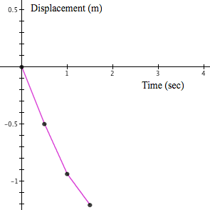
Reflection 5.1.4. Why is it important to use "number of complete ∆t-intervals from a to t" as the upper limit of the summation?
Reflection 5.1.5. How does the term $r(t)(t-\mathrm{left}(t))$ in Equation 5.1.5 represent "accumulation so far in the current $\Delta t$-interval"?
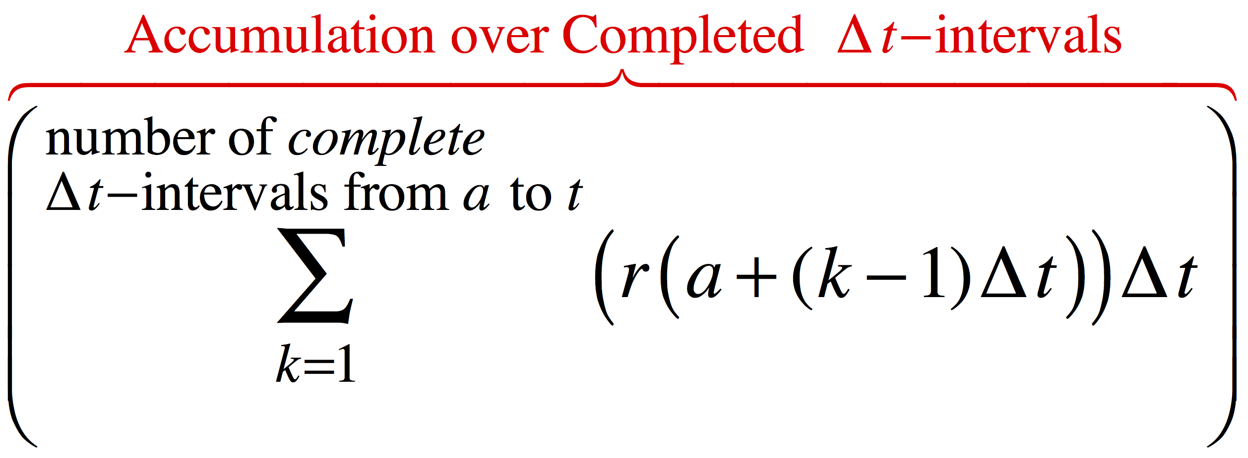
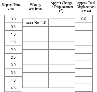
For Questions 1 - 3. Consider the video below. It shows a ball hanging from a board by a rubber cord. The ball hangs at rest 10 feet below the board. At $x = 0$ seconds, the ball is set in motion with a quick shove downward, causing the rubber cord to stretch and the ball to bounce. The graph shows the rate of change of the ball's displacement from rest with respect to elapsed time, which is the velocity function $v(x) = -\mathrm{cos}(x)$.
| Value of a |
Value of x |
∆x | No. of complete
∆x-intervals between a and x |
|
| a) | 2 | 17 | 0.03 | |
| b) | 3.2 | 5.23 | 0.0125 | |
| c) | -3 | -1.2 | 0.025 | |
| d) | -1 | -5 | 1.2 | |
| e) | 5 | 128.3 | 0.2 |
We made a mistake on the velocity function! It is actually $$r_h(t) = 15 \frac{2^{t-10}}{2^{t-10}+1}.$$
a) What needs to be changed in the system of statements that describe how to calculate approximations of the rocket’s height for values of elapsed time?
b) What would the graph of elevation relative to elapsed time look like now?
 Solution
 Solution
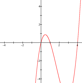 Solution
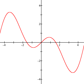 Solution
| < Previous Section | Home | Next Section > |