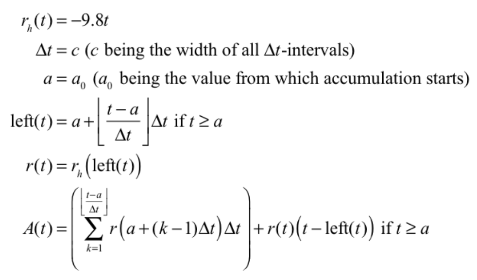
Equation 5.3.1. Approximating h(t) for any value of t given h's exact rate of change function $r_h$.
| < Previous Section | Home | Next Section > |
The goal of this section is to define an exact net accumulation function given its exact rate of change function. To this point we developed a method for approximating an exact rate of change function’s exact net accumulation function (see Equation 5.2.6).
Values of the function A that we constructed are approximately equal to the exact net variation in values of the function f for every value in f’s domain at which f has a rate of change at a moment. We do not know the function f, but by knowing its exact rate of change function $r_f$ and the initial value of f, we are able to create an approximation of f by re-creating how values of f accumulate.
A reasonable question is, "How well do values of A approximate the net variation in values of f given any value of $\Delta x$?"
In the highway elevation example of Section 5.2 it would be reasonable to say that approximations that are within 1 meter of the actual elevation are close enough. That would mean that if our approximations stop changing in the ones place once $\Delta x$ becomes smaller than some value, then that value is small enough to give approximations that are close enough to the exact value of f at that value of x.
Figure 5.3.1 uses the function round defined as $$\mathrm{round}(x,n)=\frac{\lfloor 10^n x+0.5 \rfloor}{10^n}$$ to round numbers to n decimal places. For example, $\mathrm{round}(152.3974, 2) = 152.40$, and $\mathrm{round}(152.3974, -1) = 150$.
Figure 5.3.1 shows that the value of A(1.5) rounded to 0 decimal places (to the nearest 1) stops changing when $\Delta x$ becomes less than about 0.008. So it appears that $\Delta x=0.007$ km is small enough for $1243+A(1.5)$ to be within 1 meter of $f(1.5)$. Given that $f(1.5)$ is within 1 meter of $1243+A(1.5)$, or 1308 meters, this means that we are within $\frac{1}{10}$ of 1% of the actual value of f. Notice that we can make this claim without knowing the actual value of f.
One issue that you will address in the exercises is whether a value of $\Delta x$ that produces a "close enough" value for A(1.5) also produces "close enough" values of A for other values of x.
While we will not delve into this issue in detail, the "goodness" of our approximation for a given value of $\Delta x$ depends on how rapidly the rate of change function varies within completed $\Delta x$-intervals. The more that $r_f$ varies, the smaller $\Delta x$ must be so that it is unproblematic to assume that $r_f$ is constant over $\Delta x$-intervals.
Put slightly differently, the more that $r_f$ varies over an interval, the more problematic it is to assume that $r_f$ is constant over that interval and hence the more problematic it is to assume that f is essentially linear over that interval.
Another perspective on "close enough" is when we seek a graph of an approximate accumulation function that is close enough to the graph of its exact accumulation function for us to understand the exact accumulation function’s behavior. To understand this graphical notion of "close enough" we’ll examine the case of an object falling under the influence of gravity.
Free-falling bodies near the earth’s surface accelerate at -9.8 (m/sec)/sec. The value -9.8 ignores air resistance. The unit (m/sec)/sec means that we are tracking the object’s velocity in m/sec with respect to the number of seconds it has accelerated.
A positive acceleration means the object's velocity is increasing. It does not mean the object is going up. A negative acceleration means the object's velocity is decreasing. It does not mean the ball is going down.
Suppose the object is a metal ball. The fact that the ball accelerates at -9.8 (m/sec)/sec every moment of free-fall means that its velocity after t seconds has varied $-9.8t \text{ m/sec}$.
Let h be the function that relates the ball’s upward displacement from a given reference point with the number of seconds elapsed since the ball had a velocity of 0. The rate of change of h with respect to t after t seconds have elapsed is $r_h(t) = -9.8t$. That is, the ball's rate of change of displacement from its reference point with respect to the number of seconds accelerated is $r_h(t) = -9.8t$.
A velocity of 0 at a moment does not mean the ball had a displacement of 0 at that moment. The ball could have any displacement from its reference point at a moment its velocity is 0.
The function $r_h$ is the exact rate of change function for h. The fact that $r_h(2.3)=-22.54$ means that after 2.3 seconds, the ball’s displacement at that moment varies at the rate of $-22.54 \text{m/sec}$. "At that moment" means there is some interval of width $\Delta t$ that includes 2.3, and the ball’s height varies at an essentially constant rate of $-22.54\,\text{m/sec}$ over that interval of time.
Put another way, $r_h(2.3)=-22.54$ means the variation in the ball’s displacement from its reference point is $-22.54\,dt$ meters for values of $dt$ between 0 and $\Delta t$.
We can use the method developed in Section 5.2 to approximate h, the function that gives the ball’s exact displacement from its reference height at each value of t.
The statements for this approximation of h are in Equation 5.3.1. Download the GC file containing them by clicking here.
Figure 5.3.1 shows GC’s display of $y=A(x), x≥a$, with various values of $\Delta x$ and various values of a. Two things change within the animation in Figure 5.3.1: (1) The value of $\Delta t$ varies from 1, to 0.5, to 0.1, to 0.01 for a given value of a, and (2) the value of a varies from 0, to 2, to -1, to -3. We will discuss these two aspects of Figure 5.3.1 separately.
Figure 5.3.2 starts with $a=0$ and $\Delta t=1$. The piecewise linearity of A is evident. The animation then transits to $a=0$ and $\Delta t=0.5$, $a=0$ and $\Delta t=0.1$, and then $a=0$ and $\Delta t=0.01$.
The displayed graphs of $y=A(x)$ become smoother, and successive displayed graphs change less and less. The shape of the graph of $y=h(x)$, the graph of the exact accumulation of displacement with respect to time that $ y=A(x)$ approximates, is clear. It starts at 0, decreases, and decreases faster with passing time. This makes perfect sense. As the metal ball falls, its speed (the absolute value of velocity) increases, so its distance fallen increases in successive $\Delta t$-intervals.
Figure 5.3.2 then displays the graph of $y=A(x)$ when $a=2$. Putting aside for the moment what $a=2$ might mean, the behavior of $y=A(x)$ again shows a definite a tendency to a smooth graph as $\Delta t$ becomes smaller. Similarly for $a=-1$ and for $a=-3$. The graphs of $y=A(x)$ appear smoother and the graphs appear to change less as $\Delta t$ becomes smaller.
Figure 5.3.3 displays the graphs of $y=A(x)$ grouped by value of a. The first row shows $a=0$ with various values of $\Delta t$, the second row shows $a=2$ with various values of $\Delta t$, the third shows $a=-1$, and the fourth row shows $a=-3$.
| a) |  |
| b) |  |
| c) |  |
| d) | 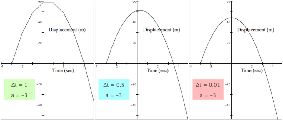 |
Figure 5.3.3. Approximate displacement functions $y=A(x),\,a\le x$ for $r_h(t)=-9.8t$
with various values of $\Delta t$ and various values of a.
Each row of Figure 5.3.3 illustrates the same tendency as we saw in Figure 5.3.2, that the displayed graphs of $y=A(x)$ became smoother as $\Delta t$ became smaller.
This illustrates the second aspect of "close enough". Letting $\Delta t=0.01$ is sufficient for us to have a clear idea of the behavior of h, the exact net displacement function generated from $r_h(x)=-9.8x$ and $a=a_0$.
We must understand what it means that $a=0$ to understand the meaning of $a=a_0$ for $a_0\neq 0$.
In the metal ball example, the value $t=0$ is the moment the ball's velocity is 0. It is not the moment we began recording variations in the ball's displacement. Keep in mind that the ball's velocity varies at the rate of $-9.8\text{ (m/sec)/sec}$ regardless of when we start recording variations in its displacement.
The value of a in the ball example is the number of seconds before or after the ball's velocity is 0 that we began recording accumulated variations in the ball's displacement.
We need not start recording accumulated variations in h when t is 0. The meaning of $t=0$ is that we establish a reference time, and the meaning of a is the number of seconds before or after this reference time that we begin recording accumulated variations.
But we must also keep in mind that $r_h(a)$ is the ball’s velocity at $t=a$. That is, at $t=0$ the ball is momentarily at rest: $r_h(0)=0$ no matter the value of a.
In Row b of Figure 5.3.3, $a=2$ means only that we started recording accumulated variations in displacement 2 seconds after the ball had a velocity of 0. At the moment $t=2$, we begin recording accumulated displacements, so $h(2)=0$ because no displacements have accumulated. Zero seconds have passed since recording began (at $t=2$ seconds).
But the ball had a velocity of $-19.6 \text{ m/sec}$ at $t=2$. It is as if we started a video recording of the falling ball 2 seconds after the moment it had a velocity of $0 \text{ m/sec}$. The video would record how the ball's displacement varied during filming, but we would have no record of what the ball did before the video started.
In Row c of Figure 5.3.3 we see that $a=-1$. This value of a means that we started recording the ball’s displacement 1 second before the ball's velocity was 0. Given the ball's velocity varied at $-9.8 \text{ m/sec}$ during the one second preceding $t=0$, the ball must have had a positive velocity in the second prior to $t=0$.
Row d of Figure 5.3.3 illustrates the discussion of Row c more vividly. We leave it for you to explain Row d in the same way we explained Row c.
In short, the meaning of a value of a is that it is the moment in h’s domain where we start recording accumulated variations in the value of h or in the value of any function that approximates h.
When we graph the net accumulation function and decrease the value of a, we see more of the accumulation function's graph, taking into consideration that $A(a)=0$. When we graph the net accumulation function and increase the value of a, we see less of the accumulation function's graph, taking into consideration that $A(a)=0$.
$A(x)$ approximates the accumulation that accrues starting from $x=a$. This means that $A(a)$ is always 0. This makes sense since at $x=a$ there has been no accumulation from a.
We must add the accumulation in f that occurred up to $x=a$ if we are to end with an approximate accumulation function for the exact accumulation function f at a value of x. But the accumulation in f up to $x=a$ is simply $f(a)$. Hence, for any value of x, $f(x)\approx f(a)+A(x)$.
We saw this in the Elevation from Rate example. The elevation function E was approximated by (elevation at the border) + (accumulated variations in elevation from the border).
The number 1243 was the value of $E(0)$, when $x=0$ km from the border. So the approximate elevation was $1243+A(x)$ meters at x meters from the border.
It is often the case that we do not know the initial value of accumulation. In those cases all we can do is approximate accumulated variations from the initial value of x, and therefore we can at best say that $f(x)\approx f(a)+A(x)$, where $f(a)$ is the accumulation function’s (often unknown) value at $x=a$.
1. Download this file and use it for parts (a)-(d) of this question. Adjust the scale of either set of axes as necessary.
2. Download this file and use it for parts (a)-(d) of this question. In each part, move the $\Delta x$ slider and observe GC’s displayed graph. Explain the effect of values of $\Delta x$ on the behavior of $y=r(x)$ and the behavior of $y’=A(x’)$.
It is worth revisiting the distinction between accumulation and net accumulation.
We explored the idea of "close enough" approximations to an exact net accumulation function in Section 5.3.2. We settled the question of "close enough" to understand that "close enough" depends on the precision you need for your present purpose.
Given that today's computers have 64-bit operating systems, computers can represent numbers only to 19 significant base-ten digits.
Round-off errors build up every time a computer adds two numbers, so at some point "close enough" becomes the practical matter that there is a limit to the computations that our computers can perform accurately.
Although we cannot compute accumulation functions exactly, we can nevertheless represent exact net accumulation functions for exact rate of change functions.
When we start with an exact rate of change function we can, in theory if not in practice, make $\Delta x$ so small that making it any smaller has no discernable effect on the value of $A(x)$, our approximation of the exact net accumulation from a to x.
We shall use the notation $A_f(x)$ to represent f's exact net accumulation from a to x. Using the accumulation function's name as a subscript follows the convention we use for differentiating between approximate and exact rate of change functions.
When $r_f$ is an exact rate of change function, any value $r_f(x)$ is an exact rate of change of f at the moment x.
The function f having an exact rate of change of $r_f(x)$ at a value of x means that f varies at essentially a constant rate of change over a small interval containing that value of x.
This means that we can, in theory, approximate the variation in f around that value of x to any degree of precision. We just need to make $\Delta x$ small enough so that $r_f(x)dx$ is essentially equal to the actual variation in f as $dx$ varies from 0 to $\Delta x$ over that $\Delta x$-interval.
The standard mathematical representation for the exact net accumulation over an interval from a to x of the function f that comes from the exact rate of change function $r_f$ is $$\int_a^x r_f(t)dt.$$
This representation of exact net accumulation from exact rate of change entails all the meanings in our representations of approximate accumulation functions.
Read the statement $A_f(x)=\int_a^x r_f(t)dt$ as, "$A_f(x)$ is the accumulation of $r_f(t)dt$ as t varies by $dt$ through every moment from $t=a$ to $t=x$.
There is a way to envision the definition of an approximate accumulation function in relation to the definition of an exact accumulation function.
When $\Delta x$ becomes infinitesimally small, the sum turns into a hyper-sum, which in turn sums the current accumulation as t varies. As the value of t varies, the value of dt varies through infinitesimilly small intervals.
It is important to have an image of how x and t vary in $A_f(x)=\int_a^x r_f(t)dt$. In one sense, we take t as a variable and turn x into a parameter whose value varies.
For each value of x in the domain of $r_f$, t varies from a to x, and the accumulated variations in $r_f(t)dt$ as t varies produce the value $A_f(x)$.
The power of integral notation is that it embodies all the features that of our method for constructing the approximate accumulation function A.
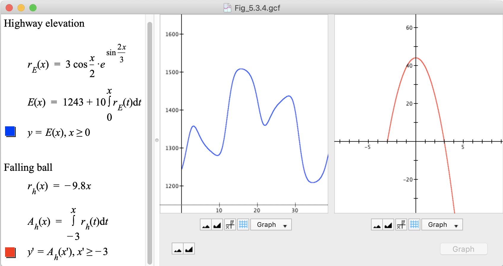
Figure 5.3.4 shows integral solutions to the problems in Sections 5.2.3 (Elevation from Rate) and 5.3.1 (Falling Metal Ball). Enter these equations into GC to practice using integral notation. Type ctrl-shift-I to get the integral sign in GC, or select Math/Integral. Press the tab key to move among the parts of the integral.
Study the definitions of E and h in Figure 5.3.4. Compare them to the approximate solutions in Sections 5.2.3 (Highway Elevation) and 5.3.1 (Falling Metal Ball) above. You should see all the details of the approximate accumulation function within the integral that represents the exact accumulation function.
It takes awhile to appreciate the economy of integral notation. As we stated, all the details of our method of approximation are entailed in integral notation.
Put another way, the integral notation is self-contained. You don’t need to assign a value to $\Delta x$ or define auxiliary functions like $\mathrm{left}(x)$ as we did prior to the definition of the approximate accumulation function. Moreover, GC can compute an integral's values when given a definition of $r_f$ and a value of a.
Integral notation has an added feature. It represents an exact accumulation function, in open form.
An open form definition of a function is one that gives a conceptual outline of the function’s meaning, but it does not give specific instructions for computing the function’s value in a definite (finite) number of steps.
A function is defined in closed form if its definition tells us how to compute values of the function in a finite number of operations on values of variables or on values of familiar functions. Chapters 6 and 9 address obtaining accumulation functions in closed form from rate of change functions in closed form.
Answer Exercise 5.2.4, part (d), using integral notation.
Density of a material at a point is defined as the rate of change of mass with respect to volume. The density of a concrete block at a point in its interior is 67 kg/$\mathrm{cm^3}$. This means that if a small cube around that point were to increase in volume by 0.001 $\mathrm{cm}^3$, the mass within that volume would increase by (67)(0.001) kg.
A concrete beam is painted on one end. It has uniform density in any cross section, but the density of the cross sections varies with distance from its painted end. The beam is 10m long and has a cross-section of 12cm x 5 cm. The rate of change function for the beam’s mass with respect to its distance from its painted end is $r_m(d) = 67+12\cos(3d)\sin(4d) \text{ g/cm$^3$},\, 0\le d\le 10$ meters.
(Adapted from Briggs & Cochran, Ch. 6.1, Problem 57).
| < Previous Section | Home | Next Section > |