| < Previous Section | Home | Next Section > |
It is worth considering the distinction between accumulation and net accumulation. If F is an exact accumulation function, then A(x) for any value of x gives an approximate value of the accumulating quantity at that value of x. All of it.
In the situations we have dealt with, we developed a method for approximating the accumulation of quantities from some starting point. These approximations are the net accumulation in the quantity -- the accumulation from the reference point to a value of x, not just the positive accumulation up to the value of x.
Put another way, the accumulation in a quantity from a starting point a to a value of its independent variable is the quantity's net accumulation, or net variation in accumulation. The function A we developed in Section 5.1 approximates $F(x)$--the net variation in accumulation from a to x.
In Section 5.1 we gave conceptual definitions of approximate rate functions and approximate net accumulation functions. Figure 5.2.0 reminds us of the way we defined the approximate rate of change function r when given an exact rate of change function $r_F$.
Figure 5.2.0 Define each value of r as $r(t)=r_F\left(\mathrm{left}(t)\right)$. Every value $r(x)$ in the graph of $y=r(x)$ is the value of $r_F$ at the beginning of the $\Delta x$-interval containing the value of x. Every value of $A(x)$ on the graph of $y=A(x)$ is an approximation of $h(x)$ at x seconds after liftoff.
Although $r(x)$ approximates the value of $r_F(x)$, every value $r(x)$ within a $\Delta x$-interval is the exact rate of change of the approximate net accumulation $A(x)$ within that interval.
Reflection 5.2.0. Explain how it is true that "Every value $r(x)$ within a $\Delta x$-interval is the exact rate of change of the approximate net accumulation $A(x)$ within that interval."
The definitions of r, left, and A were "conceptual" because each relied on values we described in principle but did not have a way to compute. These were:
We will outline how to compute these values, and to define r, by:
Our analysis of the basketball rocket example embodies the general method of generating an approximate net accumulation function A from an exact rate of change function $r_F$.
Put another way, the functions we defined for the rocket basketball can be used in any situation where there is an unknown exact accumulation function F that we wish to approximate, and we are given F’s exact rate of change function $r_F$ (the exact rate of change of accumulation at every moment).
Values $r_F(x)$ tell us the exact rate of change of $F(x)$, the exact accumulation function, at any moment of the accumulation's’s independent variable x. Our goal is to define the approximate net accumulation function A whose values approximate the net variation in values of F that the exact rate of change function $r_F$ generates.
A first requirement is to define a function that is constant over each $\Delta x$-interval and approximates the exact rate of change of accumulation over every $\Delta x$-interval.
Given:
then:
$$\color{red}{\text{(Eq. 5.2.1)}}\qquad r(x)=r_F(\mathrm{left}(x))$$
Our purpose for defining the approximate rate function r in this way is that the value of $r(x)$ is necessarily constant as x varies through a $\Delta x$-interval regardless of how $r_F(x)$ varies.
The value of $r(x)$ for every value of x in a $\Delta x$-interval is the value of rF at the beginning of that interval.
This is important because we can compute variations in accumulation when its rate of change is constant, but not when its rate of change varies.
The value of $r(x)$ for any value of x within a $\Delta x$-interval is the value of $r_F$ at the beginning of that $\Delta x$-interval. So r is necessarily constant over ∆x-intervals, whereas $r_F$ is not necessarily constant.
With r being constant over every $\Delta x$-interval,
It is convenient to let the value of u be the left end of a ∆x-interval. The left end of the $k^{th}$ $\Delta x$-interval is $a+(k-1)\Delta x$ (you should test this statement).
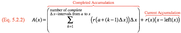
Equation 5.2.2 puts all this together in one conceptual definition. Note that "current accumulation" means accumulation within the current $\Delta x$-interval up to the value of x as x varies through its current $\Delta x$-interval. Keep in your imagination that the value of x varies, and therefore number of completed $\Delta x$-intervals and left(x) change values as the value of $x$ varies from one $\Delta x$-interval to the next!
Each value $A(x)$ is an approximation to the net variation $F(x)$--the exact accumulation from $t=a$ to $t=x$, where F accumulates variations at the rate $r_F(x)$ at each moment x.
As already noted, we lack two technical details in order to have GC compute values of $A(x)$. These are:
Remember:
There are two key ideas in computing the number of complete $\Delta x$-intervals between a and x.
The quotient $\frac{15}{3}$ being 5 tells us that 15 is 5 times as large as 3, or that there are five 3’s in 15.
Similarly, $\dfrac{33}{7}=4+\dfrac{5}{7}$ tells us that there are four complete 7’s and $\frac{5}{7}$ of 7 in 33. So an interval of length 33 contains four complete intervals of size 7.
More generally, the expression $\dfrac{x-a}{\Delta x}\text{, }x \ge a$ computes the number of intervals of size $\Delta x$ that are contained in the interval from a to x. This number includes a fractional part of $\Delta x$.
However, we want only the number of complete $\Delta x$-intervals between a and x. In other words, we want the whole number part of the quotient $\dfrac{x-a}{\Delta x}$.
The function "floor" serves this purpose. The value of floor(x), customarily written $\lfloor x \rfloor$, is the greatest integer less than or equal to the value of x. So $\lfloor 3.2 \rfloor=3$, $\lfloor 7.9999 \rfloor=7$, and $\lfloor -3.2 \rfloor=-4$.
In GC, type "floor" to get the floor function.
The number of complete $\Delta x$-intervals between a and x is therefore:
$$\color{red}{\text{(Eq. 5.2.3)}}\qquad \left\lfloor\frac{x-a}{\Delta x}\right\rfloor\text{ if } x \ge a$$
Equation 5.2.3 gives the number of complete $\Delta x$-intervals between the value of a and the value of x.
We can re-write Equation 5.2.2 as Equation 5.2.4:
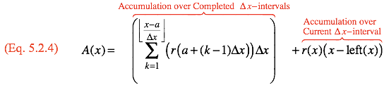
The part of A that computes accumulation over completed $\Delta x$-intervals preceding the current value of x is now defined.
We can compute the accumulation over completed $\Delta x$-intervals from a to x as the value of x varies because we now can compute the number of $\Delta x$-intervals preceding the current value of x.
The definition of $A(x)$ has the form of a linear function $y = m(x-a)+b$. $m$ is the linear function's rate of change and $b$ is the value of $y$ when $(x-a)$ is 0, or when $x=a$. In Equation 5.2.4, for any value of $x$, $b$ is the accumulation over completed $\Delta x$-intervals prior to the current value of $x$. It is constant for all values of $x$ in the current $\Delta x$-interval. $a$ is the left end of the current $\Delta x$-interval, and $m$ is $r(x)$ for all values of $x$ in the current interval. So, Equation 5.2.4 is like a dynamic linear function. It produces a different linear function for each $\Delta x$-interval because in the form $y=m(x-a)+b$, values of $m, a, \text{ and } b$ will change from interval to interval as the value of $x$ varies through its domain.
| a |
b |
$\Delta x$ | $\left\lfloor\dfrac{b-a}{\Delta
x}\right\rfloor$ |
What this value means |
| 2 | 27 | 0.03 | 833 | There are 833 complete intervals of size 0.03 within the interval that extends from 2 to 27 |
| -1.4 | 3.7 | 0.002 | ||
| 2 | -1.5 | 0.07 | ||
| 17.33 | 35.24 | 0.012 |
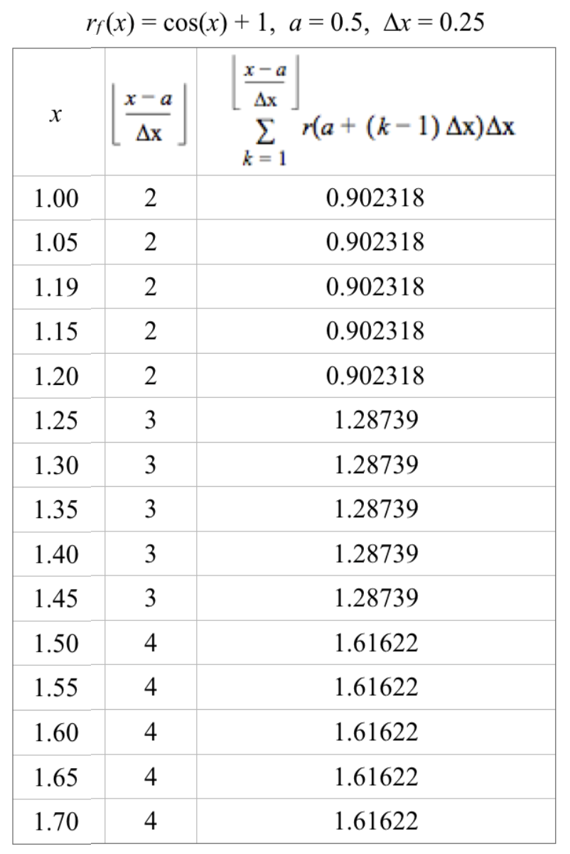
The first term in the right side of Equation 5.2.4 is $$\sum\limits_{k=1}^{\left\lfloor\frac{x-a}{\Delta x}\right\rfloor} r\left(a+(k-1)\Delta x\right)\Delta x$$
This expression computes accumulation over complete $\Delta x$-intervals prior to the current value of x.
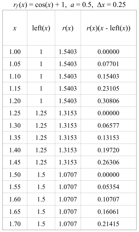
Let $r_F(x)=\cos(x)+1$, $a=0.5$, and $\Delta x=0.25$.
Notice what happens in the following table.
As the value of x varies within a $\Delta x$-interval
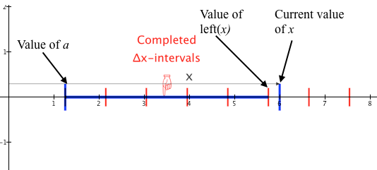
Figure 5.2.1 illustrates that as the value of x varies smoothly, the value of $$A_\text{completed}(x)=\sum\limits_{k=1}^{\left\lfloor\frac{x-a}{\Delta x}\right\rfloor}r\left(a+(k-1)\Delta x)\right)\Delta x$$remains constant within $\Delta x$-intervals. The following animation displays the graph of $y=A_\text{completed}(x)$ when $r_F(x)=\cos (x)+1$ and the value of $x$ varies through its domain.
Figure 5.2.1. The value of $A_\text{completed}(x)$ is constant within $\Delta x$-intervals.
Reflection 5.2.1 Why in Figure 5.2.1 does it appear that there is no graph for the interval $0\le x \lt 0.862$?
We have defined the part of A that computes accumulation over completed $\Delta x$-intervals that precede the current value of x.
To complete the definition of A we must compute accumulation in the $\Delta x$-interval containing the current value of x.
The computation of approximate accumulation at a constant rate over any interval is the product of the rate at which approximate accumulation changes over that interval and the length of the interval.
The approximate accumulation's rate of change over the current $\Delta x$-interval is the accumulation's exact rate of change at the beginning (left end) of the interval. The length of the partial interval is the current value of x minus the value of the interval's left end.
In short, we must create a computable definition of $\mathrm{left}(x)$.
Figure 5.2.2 shows that the value of left(x) is determined by the number of complete $\Delta x$-intervals between a and x. The value of left(x) is the value of x at the left end of the current $\Delta x$-interval, which is the value of x at the right end of the interval that extends 5 $\Delta x$-intervals from the value of a.
But 5 is the number of complete $\Delta x$-intervals between a and x. So, in Figure 5.2.2, $\mathrm{left}(x)=a+5\Delta x$.
However, Equation 5.2.3 gives us a general way to represent the number of complete $\Delta x$-intervals between a and x.
The general definition of left(x) for values of a and $\Delta x$ is therefore:$$\color{red}{\text{(Eq. 5.2.5)}}\qquad \mathrm{left}(x)=a+{\Delta x}\left\lfloor\dfrac{x-a}{\Delta x}\right\rfloor\text{ if }x \ge a$$
Equation 5.2.5 in words is, "The value of left(x) is the value of a plus the combined length of all completed $\Delta x$-intervals between a and x."
Put another way, the value of left(x) is the value of a plus the number of complete $\Delta x$-intervals between a and x times the length of one $\Delta x$-interval.
\left\ ctrl-9 x = a + $\Delta x$ * floor (x-a) / $\Delta x$ if x ctrl-shift > a
In GC-Mac, type \option-j x\ to get $\Delta x$
In GC-Windows, type \Dx\ instead of \option-j x\
Here is a video that gives another explanation of the motive for left(x) and the way to calculate it.
Sometimes GC will compute the floor of a quotient incorrectly. For example, GC will say that
$$\left\lfloor \dfrac{4.72-2}{0.01} \right\rfloor = 271$$
while it will also say that
$$\left\lfloor \dfrac{2.72}{0.01} \right\rfloor = 272$$
The two should be the same because $(4.72-2)$ is the same as 2.72. But GC says they have different values.
The problem is not with GC. The problem is that all computers have a finite number of decimal places with which to represent all real numbers. Click here to see the explanation.
Our definition of $\mathrm{left}(x)$ allows us to define the part of $A(x)$ that computes approximate net accumulation within the current $\Delta x$-interval, the interval from the beginning of the current $\Delta x$-interval to the current value of x. The statements that define $A_\text{current}$ are$$\begin{align} \mathrm{left}(x)&=a+\Delta x\left\lfloor\frac{x-a}{\Delta x}\right\rfloor\\[1ex] r(x)&=r_F(\mathrm{left}(x))\\[1ex] A_\text{current}(x)&=r(x)(x-\mathrm{left}(x)) \end{align}$$
Examine the following table. Given $a=0.5$, $\Delta x=0.25$, and $r_F(x)=\cos(x)+1$, the value of $r(x)$ is constant within $\Delta x$-intervals. This means that $A_\text{current}(x)$ starts at 0 at the beginning of each $\Delta x$-interval and increases at a constant rate within each $\Delta x$-interval.
Reflection 5.2.2. Why must it be true that $A_\text{current}(x)=0$ at the beginning of every $\Delta x$-interval?
Figure 5.2.3 shows the current accumulation within every $\Delta x$-interval starts at 0 and increases at a constant rate within each $\Delta x$-interval.
The constant rate at which accumulation increases within any $\Delta x$-interval is $r_F(\mathrm{left}(x))$, the exact rate of accumulation at the left end of the interval.
Figure 5.2.3. Graph of current accumulation within each $\Delta x$-interval as value of x varies by dx within a $\Delta x$-interval.
We now have a way to define any approximate net accumulation function for which we have an exact rate of change function. Moreover, we will define the approximate net accumulation function A so that GC can compute values of it.
Given an exact rate of change function $r_F$ whose values give the rate of change at every moment of an accumulation function , we have Equation 5.2.6:
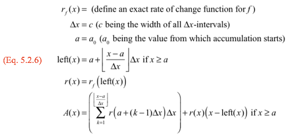
With the system of statements in Equation 5.2.6, GC can approximate any net accumulation function just by knowing its exact rate of change function.
Figure 5.2.4 gives an overview of the reasoning we used to develop the computational definition of $A(x)$, the function whose values give approximate net accumulation from exact rate of change.
Figure 5.2.4. Overview of developing the computational definition of the approximate net accumulation function given any exact rate of change function $r_F$.
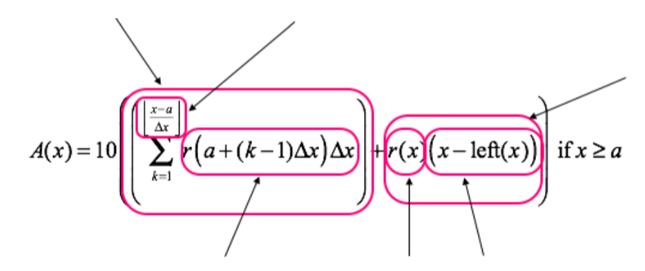
Reflection 5.2.3: Some people claim that A(x) in Equation 5.2.6 should be
$$A(x)=\left(\sum_{k=1}^{\left\lfloor \frac{x-a}{\Delta x} \right\rfloor} r_F(a+(k-1)\Delta x)\Delta x \right)+r(x)\left(x-\mathrm{left}(x)\right) \text{ if }x \ge a$$
instead of
$$A(x)=\left(\sum_{k=1}^{\left\lfloor \frac{x-a}{\Delta x} \right\rfloor} r\left(a+(k-1)\Delta x \right)\Delta x \right)+r(x)\left(x-\mathrm{left}(x)\right) \text{ if }x \ge a.$$
Are they correct? Explain. Hint: Examine $r(a+k\Delta x)$ and $r_F(a+k\Delta x)$ for a given value of $\Delta x$ and various values of a and k.
Reflection 5.2.4: Some people claim that A(x) in Equation 5.2.6 should be
$$A(x)=\left(\sum_{k=1}^{\left\lfloor \frac{x-a}{\Delta x} \right\rfloor} r\left( a+(k-1)\Delta x \right)\Delta x \right)+r_F(x)\left(x-\mathrm{left}(x)\right) \text{ if }x \ge a$$
instead of
$$A(x)=\left(\sum_{k=1}^{\left\lfloor \frac{x-a}{\Delta x} \right\rfloor} r\left( a+(k-1)\Delta x \right)\Delta x \right)+r(x)\left(x-\mathrm{left}(x)\right) \text{ if }x \ge a.$$
Are they correct? Explain.
Departments of transportation are very concerned with how steep a highway is. To qualify for federal matching funds, no stretch of highway can exceed a rate of change of elevation with respect to distance greater than 0.08 meters per meter (i.e. a rate no greater than 8/100 meter of variation in elevation per meter of highway). This rate could also be expressed as 8 m/100m or 80 m/km.
Reflection 5.2.5. Explain how a rate of change of 0.02 meters per meter, 2 meters per 100 meters, and 20 meters per kilometer are all the same rate of change of elevation with respect to distance on a road.
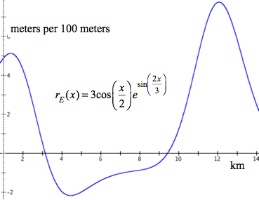
The displayed graph in Figure 5.2.4 shows a particular highway's rate of change of elevation over a stretch of road beginning at the Utah-Colorado state border. It shows the highway's rate of change of elevation (in meters of elevation per 100 meters of highway) at every distance from the border up to 14 km from the border.
This rate of change of elevation map is modeled by the function $$r_E(x) = 3 \cos (\frac{x}{2}) e^{\sin(\frac{2x}{3})}$$where a value of x is a number of km from the border.
The function $r_E$ is the exact rate of change function for the exact elevation function E. The fact that $r_E(2.3)=3.33$ tells us that 2.3 km from the border, the highway’s elevation increases at the rate of 3.33 meters per 100 meters for a brief stretch of highway around 2.3 km from the border.
Study the displayed graph of $r_E$. Its behavior by itself tells us about how the elevation varies with respect to distance from the border. Anywhere that $r_E(x)>0$, the highway’s elevation is increasing. Anywhere that $r_E(x)<0$, the highway’s elevation is decreasing. The highway’s elevation increases more rapidly wherever $r_E$ increases. The highway’s elevation decreases more rapidly wherever $r_E$ decreases.
Our goal is to define a function that approximates $E(x)$, the road’s exact elevation x km from the border as x varies from 0 to 14, given that the road’s elevation at the border is 1243 meters.
Determining elevation in this example means to compute accumulated variations in elevation, in meters, from the rate at which the elevation is varying with respect to distance along the road (in $\mathrm{\frac{m}{100m}}$). We can use the general method developed in Equation 5.2.6 to define a function that approximates the exact elevation function, which we will call E.
Equation 5.2.7 (below) is the result of specializing Equation 5.2.6 to the current situation.
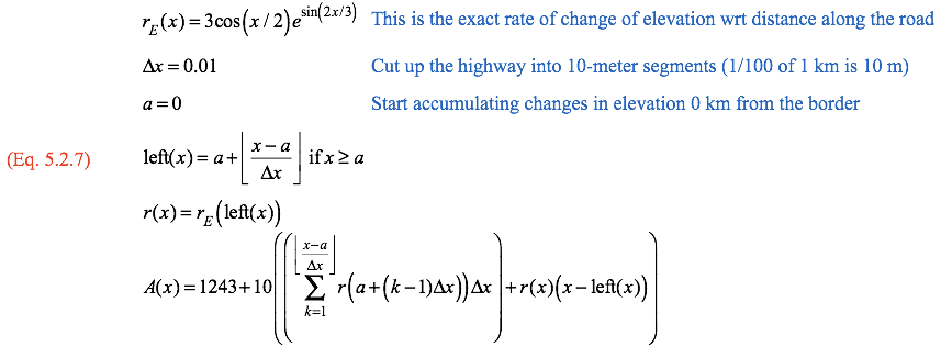
Figure 5.2.6 displays the graph of the approximate net accumulation function A, along with the GC statements that produced it. Study the GC statements in Figure 5.2.6 until you understand how each statement contributes to producing the graph displayed at the right.
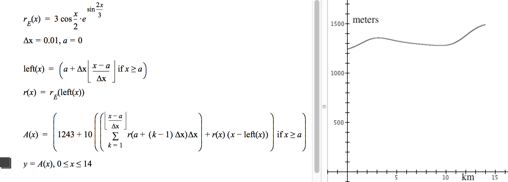
The definition of A in Figure 5.2.6 not only produces a graph of elevation in relation to distance along the highway, it gives us a way to compute net variations in elevation between specific places on the highway:
Save your GC file for this exercise. You will need it for the next exercise.
The figure below shows a ball hanging by a rubber cord. The ball is given a sharp push downward. The cord then stretches until the ball stops moving down and begins being pulled up. And so on. The ball’s rate of change of displacement (in m/sec) from its resting point with respect to elapsed time (in sec) is $r_g(x)=(0.25 \sin x-4 \cos x)e^{-0.0625x}$, where x is the number of seconds since the ball was pushed and g is the ball’s exact displacement function with respect to x.
Why does GC produce a step function as its graph of B? What is the relationship between function B and function A? Justify your answer.
$$\begin{align} r_F(x)&=0.5\left(x^2-1\right)+0.2\cos(10x)\\[1ex] a&=-1.5\\[1ex] \Delta x&=0.4\\[1ex] \text{left}(x)&=a+\Delta x \left\lfloor\frac{x-a}{\Delta x}\right\rfloor\\[1ex] r(x)&=r_F(\mathrm{left}(x))\\[1ex] C(x)&=\sum\limits_{k=1}^{\left\lfloor \frac{x-a}{\Delta x}\right\rfloor} \left(r(a+(k-1)\Delta x\right)\Delta x\\[1ex] V(x)&=r(x)(x-\mathrm{left}(x))\end{align}$$
| < Previous Section | Home | Next Section > |