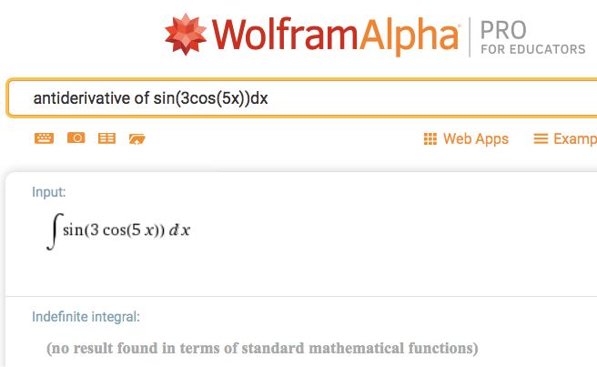
Figure 10.0.1. The result of Wolfram Alpha Pro's attempt to determine an antiderivative of sin(3cos(5x)). It could not determine one.
| < Previous Section | Home | Next Section > |
In Chapter 9 you used the Fundamental Theorem of Calculus to devise techniques for producing closed form definitions of accumulation functions that are defined in open form as integrals. The two representations (closed and open form) were equivalent.
Closed form definitions provide a formula for calculating functions' values; open form definitions remind us that accumulation functions are made by accumulating some quantity at some rate of change with respect to another quantity.
In Chapter 8, you answered questions about signed area, volume, surface area, arc length, force, work, pressure, etc. by defining accumulation functions in open form.
In Chapter 9, you found closed form definitions of accumulation functions equivalent to their definition in open form with the aim of computing their values efficiently.
It turns out that the vast majority of accumulation functions you will meet in applied settings cannot be represented in closed form. A seemingly simple case is $r_f(x)=\sin(3\cos(5x))$. Figure 10.0.1 shows Wolfram Alpha Pro's report when asked for an antiderivative of $\sin(3\cos(5x))$.
Wolfran Alpha's inability to find a closed form antiderivative of $r_f(x)=\sin(3\cos(5x))$ is not a shortcoming of Wolfram Alpha. Instead it reflects the fact that $r_f(x)=\sin(3\cos(5x))$ does not have a closed form antiderivative.
But $r_f(x)=\sin(3\cos(5x))$ does have an antiderivative! An antiderivative of $r_f(x)=\sin(3\cos(5x))$ is $$F(x)=\int_a^x r_f(t)dt$$
Why did we have you invest so much effort to learn techniques for integrating functions if they do not work on the vast majority of functions?
The answer has two parts. The first is historical. Before the advent of digital computers, mathematicians and scientists integrated functions which have closed form antiderivatives. This allowed them to calculate values of accumulation functions with reasonable effort.
The second reason for asking you to learn integration techniques is we can approximate values of functions not having a closed form antiderviative by functions that do have closed form antiderivatives.
We still face the problem that motivated Ch. 9. We must develop methods that not only give accurate approximations of accumulation functions' values, we must compute these approximations efficiently.
Section 10.1 addresses the problem of how to lessen the computational effort to approximate values of accumulation functions. In addressing this problem we also lay groundwork for Section 10.2. In this section we develop general methods for approximating values of functions we do not know how to compute.
Much of today's mathematics arose from a centuries-long quest to develop methods for computing values of common functions, such as sine, cosine, tangent, exponential, and logarithmic functions. Today we take for granted that we can evaluate them on a calculator.
Have you thought about how your calculator computes values like $\sqrt {17}$, $\cos(2.14)$, or $\left(\sqrt {15287}\right)^\left(e^2\right)$?
Before the advent of electronic digital technologies, people had to compute these values by hand. Indeed, prior to 1930 CE, a computer was "a person who calculates."
The efforts of these computers were recorded in tables of values, such as for trigonometric functions and logarithmic functions, that other computers (people) could use in their computations. Astronomers, physicists, chemists, and engineers needed these tables to make precise computations.
Sometimes tables of values were too cumbersome for quick computations. In the 1960's, engineers in NASA's project to put humans on the moon often used slide rules to quickly estimate products and quotients of large or small numbers or to estimate values of trigonometric, logarithmic, and exponential functions.
Mathematical discoveries often had their roots in the quest to make computations of functions' values more efficient. In Chapter 9 we used insights gained through the Fundamental Theorem of Calculus to find closed form representations of accumulation functions that enabled us to efficiently calculate values of open form integrals that we defined in Chapter 8.
As we saw, and will see again, there are functions not having closed form antiderivatives, such as $f(x)=\cos(x)e^{\cos(x)}$. Indeed, in a real analysis course you will learn that functions having closed form antiderivatives are exceedingly rare (have measure 0) in the class of real-valued functions.
In Chapter 10 we will develop methods for approximating values of any accumulation function, including those that cannot be defined in closed form. We also will extend these ideas and methods to create ways to compute values of functions that cannot be defined algebraically (such as trigonometric, exponential, and logarithmic functions). These latter methods are behind your calculator's ability to produce accurate computations quickly.
| < Previous Section | Home | Next Section > |