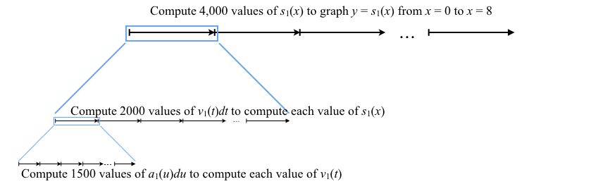
Figure 9.0.2. GC does an enormous number of calculations to display the graph of $y=s_1(x)$ from $x=0$ to $x=8$.
| < Previous Section | Home | Next Section > |
Chapter 8 was about quantifying the accumulation of quantities that accumulate at a rate of change. We repeatedly used the standard form$$F(a,x)=\int_a^x r_f(t)\,dt$$where $r_f(x)$ is the exact rate of change of an accumulation function $f$ with respect to its independent variable x, and $F(a,x)$ is the net accumulation in $f$ over the interval $[a,x]$.
Notice that in all of Chapter 8 we did not need a definition of $f$. All we needed was its rate of change function.
In Section 8.5 we modeled a situation where we were given acceleration functions for two moving objects.
We defined velocity functions in terms of acceleration functions and we defined distance functions in terms of velocity functions. The functions we defined were:
$$\color{red}{\text{(Eq. 9.0.1)}}\qquad \begin{align}a_1(t)&=0.7t+\sin\left(\frac{3\pi t}{5}\right)\\[1ex]
a_2(t)&=3-3\cos\left(\frac{2\pi t}{15}\right)\\[1ex]
v_1(t)&=\int_0^t a_1(u)du\\[1ex]
v_2(t)&=\int_0^t a_2(u)du\\[1ex]
s_1(t)&=\int_0^t v_1(u)du\\[1ex]
s_2(t)&=\int_0^t v_2(u)du\end{align}$$
Figure 9.0.1 repeats what you saw when graphing $y=s_1(x)$ and $y=s_2(x)$ in GC. It shows that GC takes a long time to display these graphs. Why?
Think about why GC takes so long to display these graphs before reading on.
For GC to calculate a value of, say, $s_1(4.1)$ it must calculate bits of distance $v_1(t)dt$ for many values of t from 0 to 4.1.
But to calculate a value of $v_1(t)dt$ for any value of t, GC must also calculate many values of $a_1(u)du$ for values of $u$ ranging from 0 to t.
To display the graph of $y=s_1(x)$ GC must repeat this double-variation process for all (actually, a large sample) of values of x from $x=0$ to $x=8$.
Figure 9.0.2 illustrates the above explanation graphically.
Suppose that:
GC does an enormous number of computations to compute values of $s_1$ and $s_2$. This is why it takes so long to generate the graphs in Figure 9.0.1. Therefore, the way to speed up GC's computation of specific values of an accumulation function is to reduce the number of computations it must do.
The definition of $s_1$ in closed form is $$\color{red}{\text{(Eq. 9.0.2)}}\qquad s_3(t)=\frac{0.7t^3}{6}+\frac{-25\sin\left(\dfrac{3\pi t}{5}\right)}{9\pi^2}+\frac{5t}{3\pi}$$
In a new window, define $s_3$ as in Equation 9.0.2. Enter $y=s_3(x)$ on a new line. Compare the speeds with which GC graphs $s_1$ and $s_3$. Keep in mind that $s_1$ and $s_3$ are the same function defined in two ways!
Move the "q" slider and watch the values of $s_1(q)$ and $s_3(q)$. Does this convince you that $s_1$ and $s_3$ are the same function?
This chapter (Chapter 9) is therefore about creating methods to improve the efficiency with which we calculate values of accumulation functions. It focuses on starting with a rate of change function defined in closed form and defining its accumulation function in closed form.
| < Previous Section | Home | Next Section > |