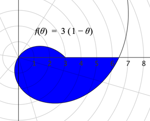
Figure 11.3.2. While the graphs of f (in Cartesian coordinates) and g (in polar coordinates) bound identical regions,
the integrals of f and g over their respective domains are not equal.
| < Previous Section | Home | Next Section>> |
The common perception of area is that all regions bounded by graphs are measured in the same way -- with rectangles that collectively approximate the region and the region's area is approximated by the sum of the rectangles' areas. An example will illustrate that this way of thinking is appropriate only when the functions graphs are displayed in Cartesian (rectangular) coordinates.
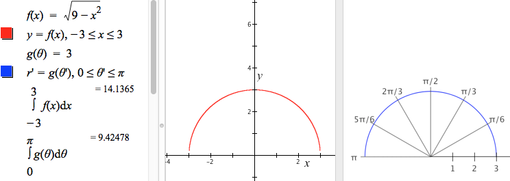
Figure 11.3.1 shows what seem to be identical regions bounded by graphs. The graph on the left is $y=f(x)$ in Cartesian coordinates, where $f(x)=\sqrt{9-x^2},-3\le x \le 3$. The graph on the right is $r=g(\theta)$ in polar coordinates, where $g(\theta)=3,0\le \theta \le \pi$.
While the regions bounded by graphs in Figure 11.3.1 appear identical, Figure 11.3.2 shows that the integrals of the functions that produce them are not identical. $\int_{-3}^{3}f(x)dx$ is approximately 14.14, while $\int_{0}^{\pi}g(\theta)d\theta$ is approximately 9.42.
The reason these two integrals have different values is this: The unsigned area of the enclosed region in the left graph accumulates at a rate of $f(x)$ with respect to x because differentials in bounded area are areas of rectangles with height $f(x)$ (see Section 8.2). The unsigned area of the enclosed region in the right graph does not accumulate at a rate of $g(\theta)$ with respect to $\theta$. Differentials in area of the bounded region are areas of sectors of a circle, not areas of rectangles.
When a region in the polar plane is bounded by the graph of $y=g(\theta)$, the function $\int_0^x g(\theta)d\theta$ gives an inappropriate measure of the enclosed region's unsigned area because it assumes an inappropriate rate of change of area with respect to $\theta$.
Figure 11.3.3 shows a closeup of the swept region in Figure 11.3.1. The area of the incremental change in swept region in Cartesian coordinates is essentially $f(x)dx$. But the area of the incremental change in the swept region in polar coordinates is not $g(\theta)d\theta$.
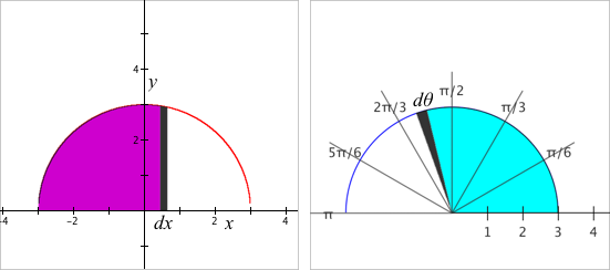
Figure 11.3.4 illustrates that when a region bounded by a circle of radius r is swept by an angle that subtends an arc of measure $\theta$ radii, the unsigned area of the swept region varies at a constant rate from 0 to $\pi r^2$ as $\theta$ varies from 0 to $2\pi$. So variations in unsigned area of swept regions in polar coordinates vary in proportion to variations in subtended arc length.
Let $A(\theta)$ be the unsigned area of a swept region in the circle of radius r. Since $A(\theta)$ varies at a constant rate with respect to $\theta$, $dA$, the differential in unsigned area, is proportional to $d\theta$, or $dA=k\cdot d\theta$ for some number k.
If we let $d\theta=\pi$ (we sweep a half circle), then $dA$ (the variation in unsigned area) is $\pi \dfrac{r^2}{2}$. Therefore, $\pi \dfrac{r^2}{2}=k\cdot \pi$, or $k=\dfrac{1}{2}r^2$. The unsigned area of a swept region in a circle with radius r varies at the rate of $\dfrac{1}{2}r^2$ with respect to variations in $\theta$. So, in a circle of radius r, $dA=\dfrac{1}{2}r^2d\theta$.
Reflection 11.3.1. Try to say in your own words why the rate of change of swept area in a circle with respect to angle measure is $\dfrac{1}{2}r^2$.
The relevance of the above to unsigned area of regions bounded by curves in polar coordinates is this (read the bullets in conjunction with viewing Figure 11.3.5):
We return to the examples of Figures 11.3.1 and 11.3.2, which suggested that the value of $g(\theta)$ is not the rate of change of unsigned area with respect to $\theta$. It is repeated below, as Figure 11.3.6--but this time with an appropriate rate of change function for unsigned area with respect to angle measure.
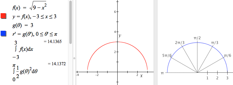
The integrals agree to two decimal places. However, we know that that the area of a semi-circle with radius 3 is $\dfrac{\pi \left(3^2\right)}{2}=14.1372$ rounded to 4 decimal places. So GC's calculation of the semicircle's area in polar coordinates is more accurate than its calculation in Cartesian coordinates.
This is because GC approximates integrals using the quadratic method developed in Section 10.1, and it has particular difficulties with the integral of a rate of change function that varies rapidly over small intervals. The function $f(x)=\sqrt{9-x^2}$ varies immensely for small variations in x near $x=-3$ and $x=3$.
Reflection 11.3.2. Attend to the independent variables in the left and right panes of Figure 11.3.6. What is the independent variable in the left pane? What is the independent variable in the right pane? How do they vary differently? Over what intervals do they vary?
Reflection 11.3.3. What signs do the areas of regions generated in Figure 11.3.6 have? Given the definition of the area of a swept region in polar coordinates as $\int_0^\theta \frac{1}{2}g(t)^2dt$, is it possible for a swept region in polar coordinates to have negative area?
Returning to Figure 11.3.5, the area of the polar region enclosed by the graph of $r=f(\theta)$ as $\theta$ varies from 0 to $2\pi$, where $f(\theta)=2(2+.2\theta\sin(7\theta))$, is $$\begin{align} A_u(0,2\pi)&=\int_0^{2\pi}\frac{1}{2}f(t)^2dt\\[1ex] &=12.3869\,\text{units}^2 \end{align}$$ to 4 decimal places.
Computing the unsigned area of the region in Figure 11.3.5 was uncomplicated. This will be true for any function f for which $f(\theta)≥0$ for all values of $\theta$ between 0 and $2\pi$.
The situation becomes more complicated when the function's graph contains bounded regions within regions. The integral $\int_a^\theta \frac{1}{2}f(t)^2dt$ will end up counting some areas more than once.
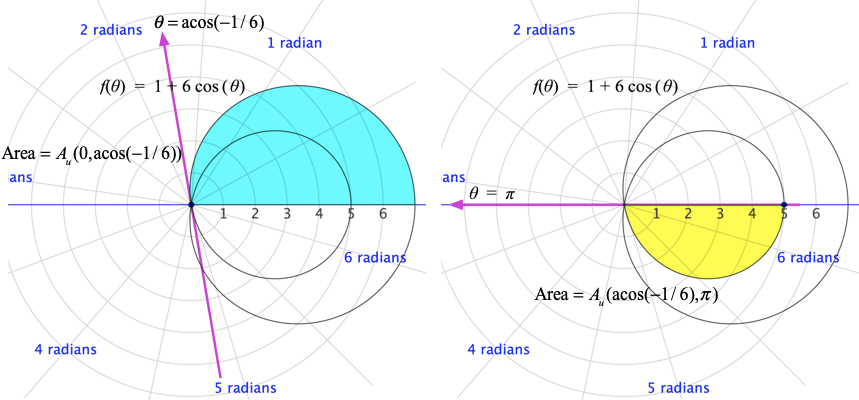
Consider the graph in Figure 11.3.7 of $r=f(\theta)$ where $f(\theta)=1+6\cos(\theta)$.
Study Figure 11.3.7 closely.
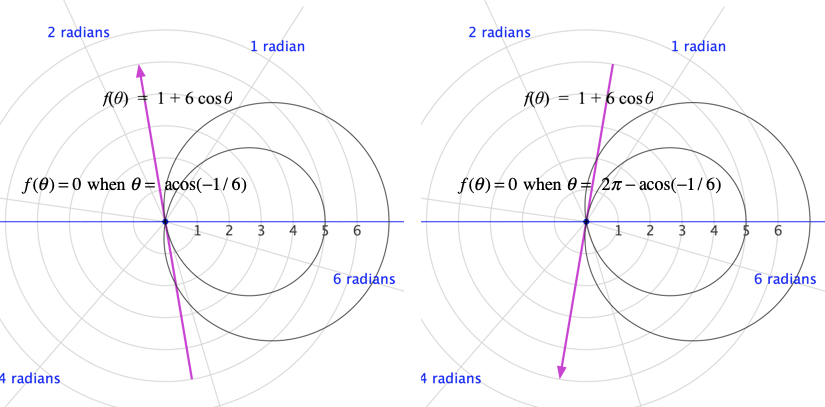
The result is that the region bounded by the graph of $r=f(\theta)$, $0\le \theta\le 2\pi$ has a subregion bounded by the graph of $r=f(\theta)$, $\acos(-1/6)\le \theta \le 2\pi-\acos(-1/6)$.
Figure 11.3.8 shows the region bounded by the inner loop being swept twice as $\theta$ varies from 0 to $2\pi$. So, the area $$\begin{align} A_u(0,2\pi)&=\int_0^{2\pi}\frac{1}{2}f(t)^2dt\\[1ex] &=59.690 \end{align}$$ counts the area bounded by the inner loop twice.
Figure 11.3.8. Region bounded by $\theta=0$ and graph of $r=f(\theta)$ as the value of $\theta$ varies from 0 to $2\pi$. The region bounded by the inner loop is swept twice: once while $f(\theta)\ge 0$ (blue) and once while $f(\theta)\le 0$ (yellow).
Figure 11.3.9 (left) shows the upper region swept as $\theta$ varies from 0 to $\acos(-1/6)$. Figure 11.3.9 (right) shows the lower inner region swept as $\theta$ varies from $\acos(-1/6)$ to $\pi$. The unsigned area of the upper region is $A_u(0,\acos(-1/6)$ and the unsigned area of the lower inner region is $A_u(\acos(-1/6),\pi)$.
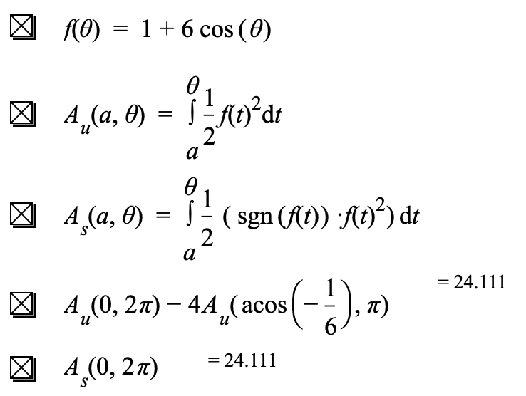
We can compute the unsigned area of the graph bounded by $r=f(\theta)$ in several ways:
It is natural to think negative values of a function should sweep negative areas in the polar plane. This is not the case for the integral $$A_u(a,\theta)=\int_a^\theta \frac{1}{2}g(t)^2dt.$$ The reason for this is $g(t)^2\ge 0$ for all values of t. We lose the sign of the function's value when squaring it. We get the same unsigned area whether the region is swept by positive or negative values of g.
However, we can capture the sign of the function in the rate of change of swept area by using the function "sgn": $\mathrm{sgn}(x)$ is called the "signum" function ("signum" is Latin for "sign"); sgn(x) produces -1 if $x\lt 0$, 0 if $x=0$, and 1 if $x\gt 0$. It is defined officially as
$$\mathrm{sgn}(x)=\begin{cases}
-1 & \text{if $x\lt 0$}\\[1ex]
0 & \text{if $x=0$}\\[1ex]
1 & \text{if $x\gt 0$}
\end{cases}$$
Given a function $g$ graphed in polar coordinates, we can recover the sign of the rate of change of swept area with respect to angle measure by multiplying $g(t)^2$ and $\mathrm{sgn}(g(t))$. The net signed area of a region in polar coordinates as $\theta$ varies is therefore $$(\text{Eq. 11.3.2})\qquad A_s(a,\theta)=\int_a^\theta \frac{1}{2}\left(\mathrm{sgn}(g(t))\cdot g(t)^2\right)dt.$$
We can test this statement against the function and graph in Figure 11.3.8.
Let $f(\theta)=1+6\cos(\theta)$. If we use $A_u(a,\theta)=\int_a^\theta \frac{1}{2}(f(t)^2)dt$ to compute the unsigned area of the outside loop (which contains the inside loop) and subtract the unsigned area of the inner loop, we should get the same result as using $A_s(a,\theta)=\int_a^\theta\frac{1}{2}(\mathrm{sgn}(f(t))f(t)^2dt$ to compute net signed area. We can test this observation by computing signed area as swept according to Figure 11.3.8 in two ways--the first by subtracting unsigned area that is included twice, and the second by computing signed area.
Figure 11.3.11 confirms that the two methods produce the same result (to 5 significant digits). The difference in unsigned areas is the same as the net signed area as $\theta$ varies from 0 to $2\pi$.
The two computations in Figure 11.3.11 give the area of the region shown in Figure 11.3.12.
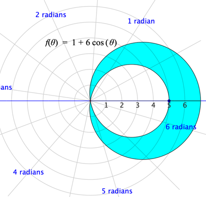
Figure 11.3.12. The region whose area is computed by the statements in Figure 11.3.11.
In GC:
| < Previous Section | Home | Next Section > |