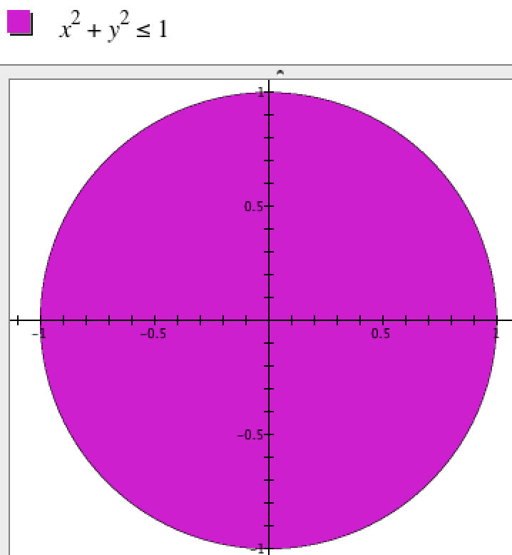
Figure 8.2.0. Typing $x^2+y^2\le 1$ into GC told it to highlight all the points in the plane whose coordinates satisfy that condition.
| < Previous Section | Home | Next Section > |
As explained in Chapter 3, GC is built to create graphs. It is designed to interpret anything you type as either a definition of a mathematical term (e.g., a function) or a command to display a graph.
Whenever you type a well-formed statement, other than a definition, GC attempts to display a graph of the ordered pairs or ordered triplets that make the statement true.
We describe regions in the plane mathematically by stating conditions coordinates of points must satisfy to be in them.
For example, the mathematical statement $\left\{(x,y)\mid x^2+y^2\le 1\right\}$, read as "The set of all points with coordinates x and y such that ...", describes the set of points in Figure 8.2.0. GC highlighted all points in the x-y plane that have coordinates x and y such that $x^2+y^2\le 1$.
Notice that in Figure 8.2.0 we typed only the condition part of the mathematical statement $\left\{(x,y)\mid x^2+y^2 \le 1\right\}$.
This is because GC always interprets any non-definitional statement involving x or y as a command to "highlight all points (x,y) such that ...".
| Statement | Meaning | Result in GC |
| $$x=3$$ | Highlight all the points in the plane with coordinates $(x,y)$ such that $x=3$ | 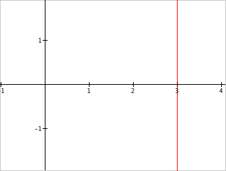 |
| $$y=x^3$$ | Highlight all the points in the plane with coordinates $(x,y)$ such that $y=x^3$. | 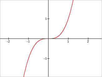 |
| $$x=y^3$$ | Highlight all the points in the plane with coordinates $(x,y)$ such that $x=y^3$. | 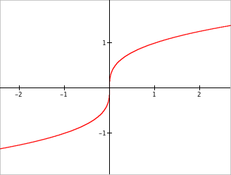 |
| $$1\le x\le 2$$ | Highlight all the points in the plane with coordinates $(x,y)$ such that $1\le x \le 2$. | 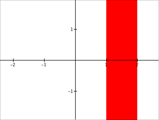 |
| $$1\le x \le 2, -0.5\le y \le 0$$ | Highlight all the points in the plane with coordinates $(x,y)$ such that $1\le x \le 2$ AND $-0.5\le y \le 0$. | 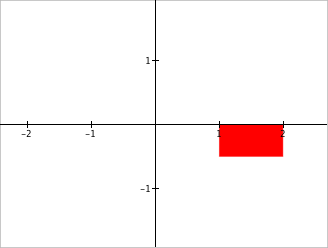 |
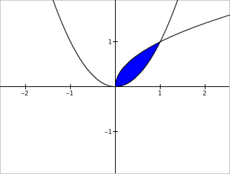
| $$f(x)=x^2\\[1ex]g(x)=\sqrt{x}\\[1ex] y=f(x)\\[1ex] y=g(x)\\[1ex] f(x)\lt y\lt g(x)$$ | * Define function $f$. * Define function $g$. * Highlight all points in the plane with coordinates $(x,y)$ such that $y=f(x)$. * Highlight all the points in the plane with coordinates $(x,y)$ such that $y=g(x)$. * Highlight all points in the plane with coordinates $(x,y)$ such that $f(x)\lt y$ and $y\lt g(x)$. |
 |
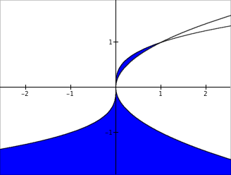
| $$f(x)=x^2\\[1ex] g(x)=x^3\\[1ex] x=f(y)\\[1ex] x=g(y)\\[1ex] f(y)\lt x \lt g(y)$$ | * Define function $f$. * Define function $g$. * Highlight all points in the plane with coordinates $(x,y)$ such that $x=f(y)$. * Highlight all points in the plane with coordinates $(x,y)$ such that $x=g(y)$. * Highlight all points in the plane with coordinates $(x,y)$ such that $f(y)\lt x$ and $x\lt g(y)$. |
 |
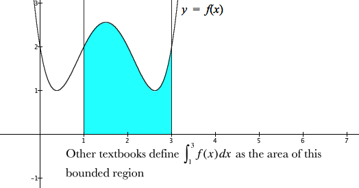
The quest to compute areas of regions played a large part in the early development of calculus.
Indeed, many textbooks define the definite integral from a to b of a function f as the area of the region bounded by $f's$ graph, the x-axis, and the lines $x=a$ and $x=b$ (see Figure 8.2.1).
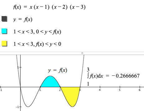
It is common to think areas are always positive (or zero). This causes a problem when defining integrals as areas of regions bounded by curves. The integral in Figure 8.2.2 is negative over the interval from 2 to 3. So, for integrals to be areas, any region below the x-axis must have a "negative" area (Figure 8.2.2).
In this textbook we have always spoken of integrals as accumulations of some quantity that accumulates at some rate of change. We avoided speaking of integrals as areas.
But this does not mean that integrals as accumulations and integrals as areas are incompatible. In this section we will explain how they are indeed compatible. But first we must look closely at the idea of signed area and its rate of change.
Examine the rectangle in Figure 8.2.3. It shows a region bounded by a rectangle that is 5 cm high and 10 cm wide.
We can think of the region bounded by the rectangle as filling from left to right as the region's width varies from 0 cm to 10 cm.
Since the area varies with width, we can ask about the area's rate of change with respect to variations in its width. Move your pointer away from the animation to make the control bar disappear.
What is the rate of change of the enclosed region's area with respect to variations in its width?
Let $w$ be the enclosed region's width as it varies. Then the value of $w$ varies from 0 to 10.
The highlighted region varies as $w$ varies, and therefore the highlighted region's area is a function of $w$, or $A(w)=5w$.
To ask about the highlighted region's rate of change of area with respect to width is to ask about $r_A$, the exact rate of change function for $A$.
The rate of change of $A$ at a moment of $w$ over an interval of length $h$ is$$\color{red}{\text{(Eq. 8.2.1)}}\qquad \begin{align} r(w)&=\frac{A(w+h)-A(w)}{h}\\[1ex]&=\frac{5(w+h)-5w}{h}\\[1ex] &=\frac{5w+5h-5w}{h}\\[1ex] &=5 \quad \mathrm{cm^2/cm} \end{align}$$
The rate of change of the rectangle's enclosed area with respect to $w$ as $w$ varies from $w=0$ to $w=10$ is 5 $\mathrm{cm^2/cm}$.
That is, the numeric value of the rectangle's height is the numeric value of the area's rate of change.
Notice that we said that the numeric value of the rectangle's height is the numeric value of the area's rate of change. The rectangle's height is not the area's rate of change. The rectangle's height is 5 cm. The area's rate of change is 5 $\mathrm{cm^2/cm}$!
There was nothing special about a height of 5 cm in Equation 8.2.1. A height of $H$ would have given us that the region's area varies with respect to width at a rate of $H \, \mathrm{ cm^2/cm}$. Indeed, a height of $f(w)$ would have given us that the region's area varies with respect to width at a rate of $f(w) \, \mathrm{ cm^2/cm}$.
To understand that a region bounded by a function's graph can have positive or negative signed area we must first be clear that function's values have directions.
Figure 8.2.3a illustrates two ways of thinking about function's values.
The first way to think about a function's values is ambiguous about how to conceive of the function's value on the graph. It is unclear whether we should:
The second way to conceive a function's value graphically clarifies the value's sign:
How to see a value of f(x)
Reflection 8.2.0. How do you anticipate that using an arrow (vector) in Figure 8.2.3a will clarify the idea of signed (negative or positive) area? What understanding does an arrow provide that a bare line segment (as in Part 1 of Figure 8.2.3a) hides?
We use the letter "d" preceding a variable to mean that the variable's value "varies a little bit".
The way to envision a differential is to first keep in mind that a variable represents the value of a quantity whose value varies. Variables vary, always.
Another key idea in understanding differentials is that they are variables whose values vary "a little bit". To vary a little bit, they must vary from somewhere. We therefore think of differentials of an independent variable as varying through fixed intervals in the variable's domain.
Finally, a differential is a variable by which another variable varies. This surely sounds confusing. Figure 4.1.1 (repeated below) illustrates this idea. The term "left(x)" in the animation means the left end of the interval containing the current value of x.
Variables and Differentials. The value of x varies smoothly through its domain. The symbols "dx" and "$\Delta x$" have differnt meanings. "$\Delta x$" represents intervals' width. "$dx$" represents how far the value of x has varied in an interval.
Reflection 8.2.1 (1) Where is $\Delta x$ in the animation? (2)The caption above says that dx and $\Delta x$ have different meanings. According to Figure 4.1.1, what are their meanings and how do they differ?
It would be understandable for you to wonder what this discussion about function's values has to do with areas of regions bounded by function's graphs. We hope that Figure 8.2.4 will help you make the connection.
In Figure 8.2.4, the region bounded by $y=0$, $x=-3$, $x=3$, and $y=2\sin(x)$ is swept out as the value of x varies from -3 to 3.
Upon zooming in, however, you see that the region is actually made of (potentially) infinitesimally-wide rectangles, and that it is the rectangles being filled that fills the bounded region.
Each rectangle has a height of $f(x)$, and is filled over an interval of length $\Delta x$ as $dx$ varies through it. Each rectangle is therefore filling at a rate of $f(x)$ $\mathrm{units^2/unit}$ throughout intervals of length $\Delta x$.
Figure 8.2.4. You can think of a region bounded by the graph of a
function as composed of rectangles of infinitesimal width. The signed
area of each rectangle varies at the rate of f(x) $units^2$ of signed area per
unit of width.
Move your pointer away from the animation to make the control bar disappear.
Reflection 8.2.2. Explain how a negative value of a function produces a negative change in accumulated signed area bounded by its graph. Explain the same for positive values of a function producing positive variations in accumulated signed area bounded by the function's graph.
We can now relate integrals as signed areas of bounded regions and integrals as net accumulation from rate of change.
Let f be a function whose graph is given within the Cartesian coordinate system.
Let A be the function such that $A(x)$ is the net signed area bounded by the graph of f over the interval $[a,x]$.
Each value of $f$ is the exact rate of change function for the signed area function $A$. So, $f(x)=r_A(x)$.
Therefore, $A(x)$ accumulates at the rate of $f(t)$ as t varies from $t=a$ to $t=x$. We say this symbolically as:
$$\color{red}{\text{(Eq. 8.2.2)}}\qquad \begin{align}
A(x)&=\int_a^xr_A(t)dt\\[1ex]
&=\int_a^x f(t)dt\end{align}$$
A region in Cartesian space bounded by the graph of a function is just a set of points. As a region, it is neither positive nor negative. But area is a measure of a region. You will see that signed area of a region can be positive or negative depending on how the region is swept out.
A region bounded by a graph is created by a function's value sweeping along the independent axis. Function's values can be positive or negative. The animation in Figure 8.2.5 illustrates this idea.
Watch the animation, then read the caption and bulleted narrative, then watch the animation again, stopping it to re-read the caption and bulleted narrative.
The animation in Figure 8.2.5 reveals the computation of the signed area of a bounded region. You compute total signed area by accumulating bits of signed area that each accumulate at a rate of change. We know very well that this accumulation is an integral over the interval $[a,x]$.
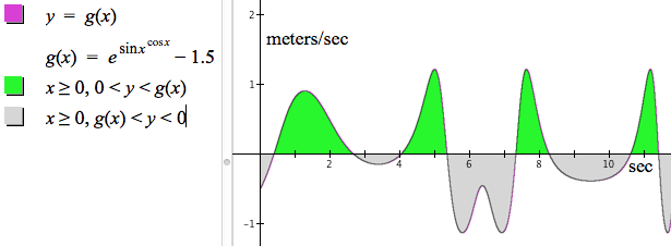
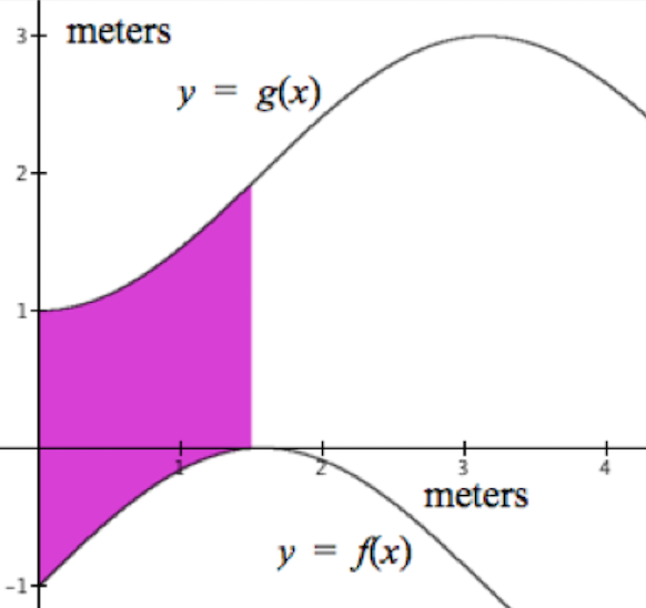
For Part 1, we must describe the regions bounded below and above the x-axis separately. Mathematically, the region above the x-axis and bounded by the graph of g is $\left\{(x,y) | x\ge 0, 0\le y\le g(x)\right\}$. The region below the x-axis and bounded by the graph of g is described mathematically as $\left\{(x,y) | x\ge 0, g(x)\le y\le 0\right\}$.
Figure 8.2.6 shows these commands and the resulting graphs in GC. In GC we need only state the conditions of the mathematical statements because GC interprets all non-definitional commands as saying, "Graph all points $(x,y)$ such that ...".
For Part 2, we need only define the integral function as shown in Figure 8.2.7.
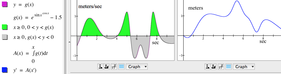
Figure 8.2.7. (Left) Graph of bounded region; (Right) Graph of
accumulation function, y=A(x).
Reflection 8.2.3. Examine each statement in the left margin of Figure 8.2.7. What does each statement do in regard to generating the graphs and highlighted regions in the two graphing panes?
Reflection 8.2.4. Examine the two graphs in Figure 8.2.7. Explain how the left graph and the right graph show the same thing in regard to accumulation of displacement in relation to number of seconds elapsed.
It is important to notice that the quantity represented by signed area in the left graph of Figure 8.2.7 does not have $\mathrm{meter^2}$ as its unit. Rather, it has meter as its unit.
Each incremental change in signed area is created by something moving at a velocity in meters/sec for a number of seconds!
This is one of the ways that thinking about integrals as areas ends up being misleading.
Area is measured in square units, whereas signed area (coming from an integral) has a unit that derives from the quantities involved.
You avoid this confusion between integrals as areas and the area having a non-area unit when you understand integrals as accumulations from rate of change.
Integrals give net signed area of regions bounded by functions' graphs. Negative signed areas and positive signed areas cancel each other to varying extents. The absolute value of a function makes all values positive, as shown in Figure 8.2.8. The absolute value function makes all regions have positive signed area.
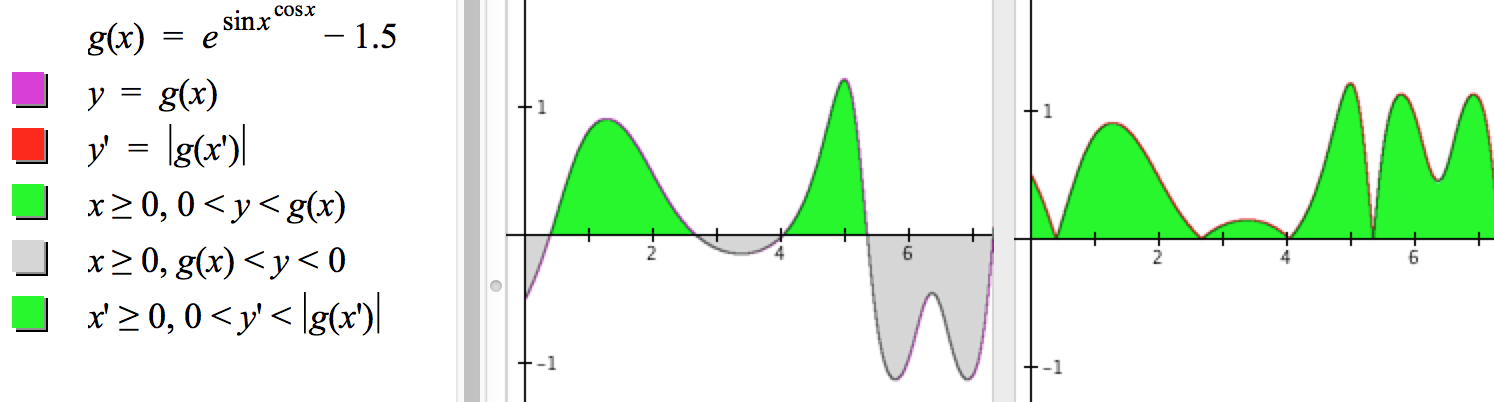
Reflection 8.2.5. The last three statements in GC produce colored regions in the displayed graphs. What regions does each statement highlight, and why does the statement highlight these regions?
Unsigned area is always positive, while signed area can be either negative or positive. Therefore an integral function that gives signed area can be increasing or decreasing over different intervals, whereas an integral function that gives unsigned area is always increasing (Figure 8.2.9).
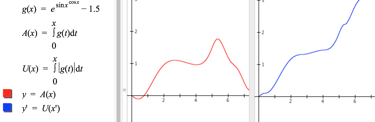
Figure 8.2.9. Graph of $y=A(x)$ (left), the signed area function, compared to graph of $y=\left|A(x)\right|$ (right).
Connect the graphs on the left sides of Figures 8.2.8 and 8.2.9 and the graphs on the right side of the same figures.
Figure 8.2.10 shows that the idea of signed area of regions bounded between functions' graphs is not as straightforward as the idea of the signed area of a region bounded by a functions graph and $y=0$ over an interval of x. The question is when to consider a region as having positive signed area and when to consider it as having negative signed area.
Figure 8.2.12. When you graph $y=f(x)-g(x)$, you are saying, "How much greater is f(x) than g(x) for values of x?" Move your pointer away from the animation to make the control bar disappear.
Figures 8.2.11 and 8.2.12 suggest that when given graphs of functions $f$ and $g$, the key to thinking about the sign of area for regions bounded between them is to decide how you are tracking them: Are you tracking how much $f(x)$ exceeds $g(x)$ or how much $g(x)$ exceeds $f(x)$?.
Figures 8.2.13 and 8.2.14 illustrate the relationship between direction of comparison between two functions and the signed area of regions bounded by their graphs.
Reflection 8.2.8. Examine the shaded regions in left and right parts of Figure 8.2.13. Must a shaded region on the left have the same signed area as the corresponding shaded region on the right? Explain.
Reflection 8.2.9. Examine the shaded regions in left and right parts of Figure 8.2.14. Must a shaded region on the left have the same signed area as the corresponding shaded region on the right? Explain.
In this entire section we have shown that the idea of integral as signed area of a region bounded by one or more graphs is entirely consistent with the general theme of this book--that an integral is an accumulation of variations in a measured quantity that varies at a rate of change with respect to another quantity.
Moreover, we demonstrated that the general idea of integral as accumulation is coherent with signed areas of regions bounded by graphs regardless of the coordinate system.
As is always the case with integrals as accumulations, the key to integrals as signed areas in any coordinate system is to determine the appropriate rate of change function whose values give the rate of change of signed area at every moment of its independent variable.
| a. | 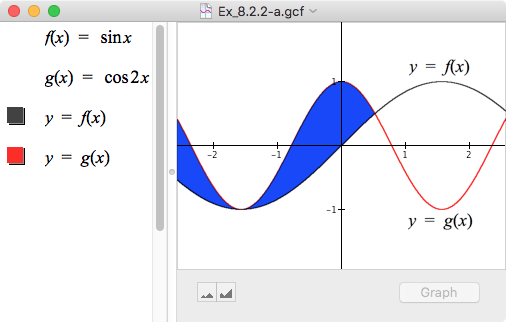 |
| b. | 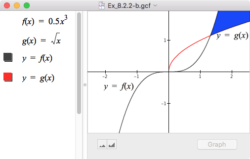 |
| c. | 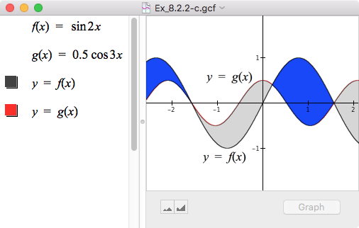 |
| d. | 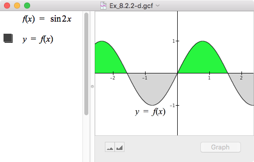 |
| e. | 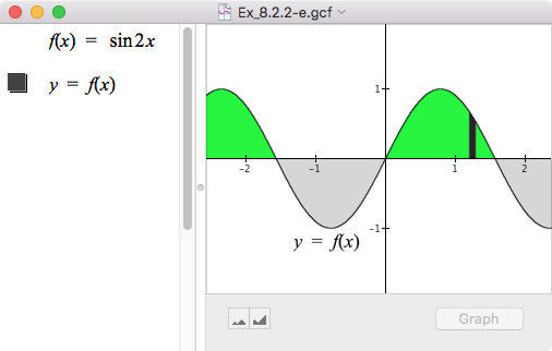 |
The function $f$ gives Stefan's displacement, in miles, to the North of his house x hours since he started walking. The function $r_f$ defined as $r_f(x)=\sin(5x)-\dfrac{x}{2.5}$ is the exact rate of change function for $f$ with respect to x.
For each of a. - d., explain the meaning in this situation of the given statement. Your answer should explain both the sign and the magnitude of the expression's value if one is given.

Bob is looking at one function $h$ and finding the net signed area bounded by its graph and the x-axis at all values of x between -3 and 7. Explain how Bob can think of this situation as finding the net signed area bounded by graphs of two functions.
| < Previous Section | Home | Next Section > |