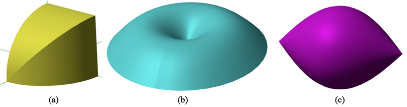
Figure 8.3.1. Examples of solids we will examine.
| < Previous Section | Home | Next Section > |
Ancient civilizations were keen to find ways to compute volumes of solids. Archimedes (287-212 BCE) derived formulas for volumes of a cylinder, sphere, and cone. Chinese mathematicians in the same period derived formulas that approximated volumes of the same solids. Cavalieri (1598-1647) devised a method for computing volumes of solids that was a precursor of modern calculus.
Computing volumes of solids was a testing ground for Newton's and Leibniz' new methods, grounded in the analysis of functions and variation in functions' values, that launched the calculus.
Newton thought of completed volumes and surface areas as having accumulated as they covaried with another quantity. Our treatment of volumes and surface areas of solids will build from Newton's approach.
To develop methods for quantifying the volume of regions in space, we will use ideas from Chapter 5 that we employed in Section 8.2 to find areas of regions in the plane.
We will define functions that model the accumulation of volume or surface area by determining the rate at which volume or surface area varies through moments of its independent variable.
It is natural to look at a solid and to think that nothing about it varies--that it is rather than it is made. Figure 8.3.1, below, shows three solids like this. They appear as complete and unmade.
Figure 8.3.1. Examples of solids we will examine.
We will use these solids to exemplify the two step process mentioned above: (1) Think of the solid as an empty shell; (2) Fill the shell in a way that supports quantifying its volume.
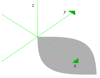
Figure 8.3.2 shows a quarter circle of radius 1 in the x-y plane. Run a square along an axis, perpendicular to the plane, so that the length of its sides is the perpendicular distance from the axis to the quarter circle. Do it again after covering the square's edges in pixie dust. The pixie dust leaves a record of everywhere each point on the square's edges has been, creating a shell that we will fill.
Figure 8.3.2 Start with a quarter circle in the x-y plane. A shell is formed by
running a square of varying width perpendicularly to the plane along an axis.
Again, the length of the square's sides in Figure 8.3.2 at any place on the axis is the perpendicular distance from the axis to the quarter circle. The shell is created by sprinkling the square's edges with pixie dust, so that the square leaves behind a trace of where it has been. The pixie dust has the effect of creating a shell that we will fill.
Figure 8.3.3 shows the graph of $y=\sin(x).\, 0\le x \le \pi$. The animation first shows the graph rotated around the y-axis, then rotated again but sprinkled with pixie dust. The pixie dust leaves a record of everywhere each point on the graph has been, creating a shell for the solid we will make by filling it.
Figure 8.3.3 Graph of $y=\sin(x)$ rotating around the y-axis, then rotated again sprinkled with pixie dust.
Figure 8.3.3 shows the graph of $y=\sin(x).\, 0\le x \le \pi$. The animation first shows the graph rotated around the x-axis, then rotated again but sprinkled with pixie dust. The pixie dust leaves a record of everywhere each point on the graph has been, creating a shell for the solid we will make by filling it.
Figure 8.3.4 Graph of $y=\sin(x)$ rotated around the x-axis, then rotated again sprinkled with pixie dust.
It is timely for us to talk about the idea of a cylinder, since we will "fill" each shape with cylinders that vary in height or radius.
A cylinder is a geometric shape that has these properties:
The volume of a cylinder is $V=A_bh$, where $V$ is the cylinder's volume, $A_b$ is the area of the cylinder's base, and h is the cylinder's height measured perpendicularly from the plane containing the base.
The surface area of a cylinder's side is $A_s=Ph$, where $A_s$ is the area of the cylinder's side, $P$ is the perimeter of the cylinder's base, and h is the cylinder's height.
Cylinders can be upright or slanted. We will employ only upright, or "right" cylinders to approximate a region bounded by a shell.
A right cylinder is a cylinder whose sides are perpendicular to its top and bottom. We will use right cylinders exclusively to fill solids.
In this chapter, we shall mean "right cylinder" when we speak of cylinders.
Figure 8.3.5, below, presents examples of right cylinders. All of them have congruent, parallel tops and bottoms with sides perpendicular to top and bottom. The volume of each is $V=A_bh$, where $V$ is the cylinder's volume, $A_b$ is the area of the cylinder's base, and h is the cylinder's height measured perpendicularly from the plane containing the base.
Figure 8.3.5. Examples of right cylinders.
Reflection 8.3.1. Attend especially to (a) and (d) in Figure 8.3.5. Explain why they are cylinders.
Reflection 8.3.2. Explain why the formula $V=A_bh$ applies to the solid in Figure 8.3.1(d) even though it has a hole in it.
It will be useful to open Figure 8.3.1 in a new window while viewing the animations in this section. Think of each shape as a hollow shell that you will fill. The animations in this section suggest ways to fill these empty shells so that we may approximate their volumes with any degree of accuracy.
Figure 8.3.6 shows the shell in part (a) of Figure 8.3.1. The animation shows it being filled with square cylinders of constant width and varying height.
As h varies along its axis, each cylinder has constant width while its height varies by $dh$ through an interval of length $\Delta h$. A new cylinder begins when the value of h passes into the next $\Delta h$-interval.
Figure 8.3.6 The shell is filled with square cylinders of constant width and varying height.
Completed cylinders are shown in magenta. Varying cylinders are shown in blue.
We use "fill" in the sense of "fill a jar with marbles". The cylinders leave empty gaps within the shell. So the volume of our fills approximates the volume of the solid within the shell.
A much smaller value of $\Delta h$ produces smaller gaps and therefore produces a more accurate approximation to the exact volume.
Figure 8.3.7 shows the shell in part (b) of Figure 8.3.1. The animation shows it being filled with circular cylinders of constant radius and varying height. As h varies along its axis, each cylinder has constant radius while its height varies by $dh$ through an interval of length $\Delta h$. A new cylinder begins when the value of h passes into the next $\Delta h$-interval.
Figure 8.3.7 The shell is filled with circular cylinders of constant radius and varying height.
Completed cylinders are shown in magenta. Varying cylinders are shown in blue.
Figure 8.3.8 shows the shell in part (c) of Figure 8.3.1. The animation shows it being filled with circular cylinders of constant radius and varying height.
As h varies along its axis, each cylinder has constant radius while its height varies by $dh$ through an interval of length $\Delta h$. A new cylinder begins when the value of h passes into the next $\Delta h$-interval.
Figure 8.3.8 The shell is filled with circular cylinders of constant radius and varying height.
Completed cylinders are shown in magenta. Varying cylinders are shown in blue.
Reflection 8.3.3 We used the word "height" for cylinders in Figures 8.3.6, 8.3.7 and 8.3.8. But the shell in Figures 8.3.6 and 8.3.8 is filled with cylinders that appear sideways. Why is it appropriate to say that the cylinders in Figures 8.3.6 and 8.3.8 have varying heights?
Figure 8.3.9 shows the shell in part (b) of Figure 8.3.1. This time, the animation shows the shell being filled with circular cylinders of constant height and varying radius.
As r varies along its axis, each cylinder has constant height while its radius varies by $dr$ through an interval of length $\Delta r$. A new cylinder begins when the value of r passes into the next $\Delta r$-interval.
Figure 8.3.9 The shell is filled with circular cylinders of constant height and varying radius.
Completed cylinders are shown in magenta. Varying cylinders are shown in blue.
Reflection 8.3.4. Figures 8.3.7 and 8.3.9 show the same shell being filled two different ways. Describe how the ways of filling the same shell differ from each other yet produce essentially the same volume for sufficiently small values of $\Delta h$.
The purpose of these exercises is for you to practice two things: conceptualize a shell and how it is made, and conceptualize a shell being filled by cylinders. You will do this by trying to imagine them and then sketch what you imagine.
You will become better at visualizing shells and fills by attempting to sketch them, no matter how well you do it. You will not become better at it by looking quickly at hints and solutions before you have made a serious effort.
Notice that f's independent variable is x while the accumulating volume's independent variable also is x. Could you have used y as the accumulating volume's independent variable? Explain.


Though the size of a cylinder can vary in many ways, we will focus on their height and radius. Figure 8.3.? shows the same initial cylinder varying in these two ways: The left animation shows the cylinder's height varying while its base remains constant. The right animation shows the cylinder's radius varying while its height remains constant.
Figure 8.3.10. Two ways that a cylinder's size can vary:
• Its height varies while its base remains constant (left), or
• Its radius varies while its height remains constant (right).
The two cylinders start in identical states, with height $h_0$, inner radius $r_0$ and outer radius $r_1$, where $r_1\gt r_0\ge 0$. The left cylinder's height in Figure 8.3.10 increased by 1. The right cylinder's outer radius increased by 1. Let's examine their variations in volume.
The initial volume of both cylinders is area of base times height. So $$\begin{align} V_\text{init}&=\left(\pi r_1^2-\pi r_0^2\right)h_0\\[1ex] &=\pi h_0 \left(r_1^2-r_0^2\right).\end{align}$$ The left cylinder's final volume after its height increased by 1 is $$\begin{align} V_L&=\pi \left(h_0+1\right) \left(r_1^2-r_0^2\right)\\[1ex] &=\pi h_0\left(r_1^2-r_0^2\right)+\pi\left(r_1^2-r_0^2\right)\\[1ex] &=V_\text{init}+\pi\left(r_1^2-r_0^2\right). \end{align}$$
The right cylinder's final volume after its radius increased by 1 is $$\begin{align} V_R&=\pi h_0 \left(\left(r_1+1\right)^2-r_0^2\right)\\[1ex] &=\pi h_0\left(r_1^2-r_0^2+2r_1+1\right)\\[1ex] &=\pi h_0\left(r_1^2-r_0^2\right)+\pi h_0\left(2r_1+1\right)\\[1ex]&=V_\text{init}+\pi h_0\left(2r_1+1\right).\end{align}$$
The cylinders' were identical at first. Their volumes began with the same value. Their volumes increased by different amounts with a change of 1 in height in the left cylinder and a change of 1 in radius in the right cylinder.
Therefore, a cylinder's rate of change of volume with respect to height and its rate of change of volume with respect to outer radius are different.
The formula for volume of a cylinder is $$V=A_bh$$where $A_b$ is the area of the cylinder's base and h is the cylinder's height.
If the cylinder's base remains constant while its height varies, then volume is a function of height, so $$\begin{align}V(h)&=A_bh,\text{ and therefore}\\[1ex]r_v(h)&=A_b\end{align}$$
This says that when a cylinder varies so that its base remains constant while its height varies, the cylinder's rate of change of volume with respect to its height has the same numerical value as the area of its base.
We emphasize "... same numerical value ..." because the cylinder's rate of change of volume with respect to height is measured in cubic units per unit while the area of the base is measured in square units. They are different quantities having the same numerical value.
To repeat, a cylinder's rate of change of volume with respect to height is $r_v(h)=A_b$. The cylinder's change in volume over any $\Delta h$-interval is therefore $A_b dh$ as h varies by $dh$ through the interval.
When the base area of a circular cylinder is constant and the cylinder's height varies, the cylinder's rate of change of volume with respect to its height is constant.
The cylinder's change in volume over any $\Delta h$-interval is $r_v(h)dh$ as h varies by $dh$ through the interval. Accumulated volume within the solid's shell as h varies from $a$ to x is therefore $V(a,x)=\int_a^x r_v(h)dh$. (See a repeat of Figure 8.3.7 here.)
Notice that we defined V with two arguments. We included the initial value of accumulation as an argument in V's definition so that we do not need to define the intial value separately, with a line $a=a_0$. The accumulation's initial value is now part of the definition of V.
Instead of writing $$a=2, V(x)=\int_a^x r_v(t)dt$$ we defined V as $$V(a,x)=\int_a^x r_v(t)dt.$$ We can then write $V(2,x)$, $V(3,x)$, etc., without having to define different starting values for different evaluations of V.
We can also make statements like $V(3,7)=V(3,5)+V(5,7)$. If we feel adventurous, we could create a 3-d surface by graphing $z=V(x,y)$ in GC.
Reflection 8.3.5. We determined that the rate of change of a cylinder's volume with respect to its height is constant, and has a numerical value that is equal to the area of its base. Examine the animation in Figure 8.3.11. Does this cylinder's volume vary at a constant rate with respect to its height?
Figure 8.3.11. Does this cylinder's volume vary at a constant rate with respect to its height?
Consider the cylinder below. The cylinder's height h and inner radius $r_0$ remain constant while its outer radius r varies.
The cylinder's volume as a function of outer radius is $$V(r)=\pi h\left(r^2-r_0^2\right)$$ where h and $r_0$ are constants.
The rate of change of the cylinder's volume with respect to its varying radius is therefore $$\begin{align}r_v(r)&=\pi h 2r\\[1ex] &=(2\pi r )h\\[1ex]&=\text{perimeter}\cdot \text{height}\end{align}$$
The value of $r_v(r)$, the cylinder's rate of change of volume with respect to its outer radius r, is $2\pi r h$.
Notice: $2\pi r h$ is the numerical value of the cylinder's outer surface area at each value of r as r varies. The cylinder's volume does not vary at a constant rate as its outer radius varies.
However, for sufficiently small values of $\Delta r$ the cylinder's rate of change of volume with respect to r is essentially constant. When $\Delta r$ has an infinitesimal value, the change in volume is essentially $r_v(r)dr$ as r varies by $dr$.
When a circular cylinder's height h is constant and the its outer radius r varies, the cylinder's rate of change of volume with respect to its outer radius is $r_v(r)=2\pi hr$.
The cylinder's variation in volume as $dr$ varies over sufficiently small $\Delta r$-intervals is essentially $r_v(r)dr$. Total accumulated volume within the solid's shell as r varies from $a$ to x is therefore $V(a,x)=\int_a^x r_v(r)dr$. (See a repeat of Figure 8.3.9 here.)
We emphasize again the phrase "...same numerical value". Rate of change of volume with respect to outer radius is measured in $\text{unit}^3/\text{unit}$. Surface area of a cylinder's outer side is measured in $\text{unit}^2$.
A cylinder's rate of change of volume with respect to radius and the cylinder's surface area as a function of radius are different quantities that have the same numerical value.
Finally, we state without demonstration two generalizations of the above development.
The animations showing different solids being filled within a Cartesian coordinate system illustrate the idea that approximate volume accumulates at an essentially constant rate as $dx$ or $dy$ varies through sufficiently small intervals of the accumulating volumes' independent variable.
Remember that an accumulating volume's independent variable is determined by the method you choose to fill the solid's shell. It need not be the same as the independent variable of the function or functions whose graphs generate the shell.
If you vary accumulated volume by varying the value of x, then x is the accumulation's independent variable. If you vary accumulated volume by varying the value of y, then y is the accumulation's independent variable.
To quantify an accumulating volume we need mathematical descriptions of the functions whose graphs generate the solid's shell. Once we have actual functions we can use an appropriate method to represent, and hence calculate, heights, widths, and radii of cylinders for the method we choose.
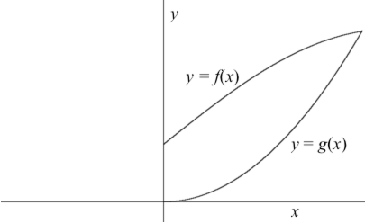
Figure 8.3.12 repeats Figure 8.3.6. The axes in Figure 8.3.6 were not named, so we can name them in any convenient way. Take the left downward axis to hold values of positive x and the right downward axis to hold values of positive y.
Figure 8.3.12. Quarter circle in the x-y plane with radius $r=1$.
Take the left downward axis to be positive x and the right downward axis to be positive y.
Completed cylinders are shown in magenta. Varying cylinders are shown in blue.
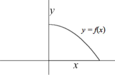
The quarter circle in Figure 8.3.12 has radius $r=1$. Its equation is $x^2+y^2=1,\,0\le x \le 1,\, 0\le y \le 1$. We can rewrite the equation to express y as a function of x, so that $y=f(x)$ where $f(x)=\sqrt{1-x^2},\, 0 \le x \le 1$. The quarter circle now is the graph of $y=f(x)$.
As the solid's accumulating volume varies, a square cylinder in blue is the only one that is varying in volume. It becomes magenta when it is "complete", after x (and hence $dx$) has varied through that $\Delta x$-interval.
A cylinder has a constant base area as x varies within the cylinder's $\Delta x$-interval. The base is a square with sides of length $f(x_b)$, where $x_b$ is the value of x at the beginning of the cylinder's $\Delta x$-interval. The cylinder's base area is $\left(f(x_b)\right)^2$.
The rate of change of volume with respect to height for a square cylinder is therefore $r_v(x)=\left(f(x)\right)^2$ for each value of x within a $\Delta x$-interval.
For sufficiently small values of $\Delta x$, the accumulated volume within a cylinder is $r_v(x)dx$ as the cylinder's height $dx$ varies. The total accumulation of volume from $a$ to x will therefore be $V(a,x)=\int_a^x r_v(t)dt$, or $$\begin{align}V(a,x)&=\int_a^x r_v(t)dt\\[1ex] &=\int_a^x \left(f(t)\right)^2dt\\[1ex] &=\int_a^x \left(\sqrt{1-t^2}\right)^2dt\\[1ex] &=\int_a^x\left(1-t^2\right)dt\end{align}$$
Because we defined $r_v(x)=\left(f(x)\right)^2$ and defined f as $f(x)=\sqrt{1-x^2}$, the first line of the above equation would have been sufficient to define $V(a,x)$. The remaining lines simply substitute the definitions of $r_v$ and f.
The left side of Figure 8.3.13 shows volume accumulating over infintesimal $\Delta x$-intervals. The right side shows the graph of accumulating volume as the value of x varies from 0 to 1.
Figure 8.3.13. (Left) The solid's volume accumulates smoothly as x varies from 0 to 1.
(Right) the graph of $V(0,x)$ as x varies from 0 to 1.
Figure 8.3.14 repeats the graphs from Exercise 6 of Exercise Set 8.3.1. In this figure, $\,f(x)=1+\sin(x/2.5)$ and $g(x)=x^2/4$. The animation shows the cylinders that will fill the shell that these graphs make when rotated around the y-axis.
While varying, the cylinders have a constant height and a varying outer radius. The cylinder's height throughout each $\Delta x$-interval is the value of $f(x)-g(x)$ at the beginning of the interval. The outer radius is the value of x as x varies by $dx$ through the $\Delta x$-interval.
The volume of each cylinder (and thus of the accumulating volume) for infitesimal values of $\Delta x$ varies at a rate that is equal to the cylinder's outer surface area, which is $perimeter\cdot height$, or $(2\pi x)\left(f(x)-g(x)\right)$.
Figure 8.3.14. One cylinder varying in radius as x varies by $dx$ through each $\Delta x$-interval.
The graphs' point of intersection, determined graphically in GC, is $(3.4424,2.9625)$ to four decimal places.
Reflection 8.3.7. Explain why the height of each cylinder at the beginning of its $\Delta x$-interval is $f(x)-g(x)$.
Figure 8.3.15 adds two details to the discussion of Figure 8.3.14. First, it shows that the accumulating volume varies by $r_v(x)dx$ as x varies by $dx$ through $\Delta x$-intervals of infinitesimal length. Second, it shows that the function that evaluates accumulated volume from 0 to x is $V(0,x)=\int_0^x r_v(t)dt$. The graph on the right is of $y=V(0,x)$ as the value of x varies.
Figure 8.3.15.
Reflection 8.3.8. As noted in Figure 8.3.14, the x-coordinate of the graphs' point of intersection's is 3.4424. Use this fact, and the definition of $V$, to determine the total accumulated volume as x varies from 0 to 3.4424.
Figure 8.3.16 repeats the graphs from Figure 8.3.14 with f and g defined as $f(x)=1+2\sin(x/2.5)$ and $g(x)=x^2/4$. We again rotate the graphs around the y-axis. This time, however, we will fill the solid's shell with cylinders by letting y be the accumulating volume's independent variable.
Figure 8.3.16. The cylinder's height is $dy$ as y varies through a $\Delta y$-interval. The cylinder's width is the distance between the graphs at the beginning of the $\Delta y$-interval.
The cylinder's height is $dy$ as y varies through a $\Delta y$-interval. The cylinder's inner radius and outer radius are values of x. It requires an explanation to understand this clearly. Refer to Figure 8.3.17 for the following discussion.
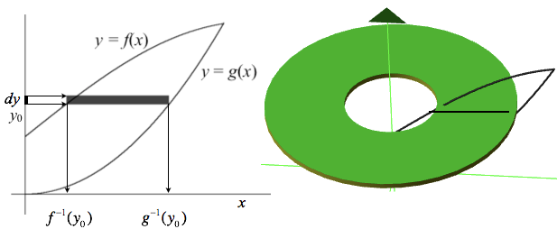
Figure 8.3.17. Two views of a the cylinder that varies in Figure 8.3.16: Its appearance in 3 dimeinsions (right) and
the cylinder's relationships with graphs of $y=f(x)$ and $y=g(x)$.
Figure 8.3.17 shows two views of the cylinder that varies in Figure 8.3.16. The left side shows that the cylinder's height is $dy$ as y varies through a $\Delta y$-interval that begins at $y=y_0$.
It also shows that the inner circle has radius $f^{-1}(y_0)$ for the value of y at the beginning of a $\Delta y$-interval and its outer radius is $g^{-1}(y_0)$. The right side shows that the area of the cylinder's base is the area of circle bounded by the outside circle, including the hole, minus the area of the hole bounded by the inside circle. Why are we concerned with the area of the base? Because the area of the base is the rate of change of volume with respect to height of a cylinder whose base is constant while its height varies.
The cylinders in Figure 8.3.16 all have a constant base and varying height. The accumulating volume's rate of change is therefore the cylinder's base area. However, to determine the base area we must define inverse functions for f and g.
We must determine the function h so that $h(y)=f^{-1}(y)$ for $f(x)=1+2\sin(x/2.5),\, x\ge 0\text{ and }y\ge 1$. We do this by solving for x in terms of y: $$\begin{align} y&=1+2\sin\left(\frac{x}{2.5}\right)\\[1ex] y-1&=2\sin\left(\frac{x}{2.5}\right)\\[1ex] \frac{y-1}{2}&=\sin\left(\frac{x}{2.5}\right)\\[1ex] \mathrm{asin}\left(\frac{y-1}{2}\right)&=x/2.5\\[1ex] 2.5\mathrm{asin}\left(\frac{y-1}{2}\right)&=x\\[1ex] h(y)&=2.5\mathrm{asin}\left(\frac{y-1}{2}\right) \end{align}$$
For a given value of $y\ge 1$ in the range of f on the y-axis, the value of $h(y)$ is the value of x on the x-axis such that $f(x)=y$.
We also need a function k so that $k(y)=g^{-1}(y)$ for $g(x)=x^2/4$, $x\ge 0$. This is easy: $$\begin{align}y&=\frac{x^2}{4}\\[1ex] 4y&=x^2\\[1ex] \sqrt{4y}&=x\\[1ex] k(y)&=\sqrt{4y}\end{align}$$
Reflection 8.3.9. Define f, g, h, and k, as given, above in GC.
Refer again to Figure 8.3.17. The area of the outer circle, including the hole, of any cylinder is $\pi k(x)^2$. The area of the inner circle, bounding the hole must be defined in two parts: for values of y such that $0\le y \le 1$ (there is no hole) and for values of $y\gt 1$ for which $x\gt 0$ (there is a hole). We'll define a new function j so that $j(y)=0$ if $0 \le y \le 1$, $\, j(y)= h(y)$ if $y\gt 1$. $$j(y)=\begin{cases} 0 & \text{if $0\le y \le 1$}\\[1ex]h(y) & \text{if $y\gt 1$}\end{cases}$$
The rate of change of volume with respect to height for any cylinder is the area of the cylinder's base. We therefore define $r_v$ as $$r_v(y)=\pi \left(k(y)^2-j(y)^2\right).$$
For sufficiently small values of $\Delta y$, the volume of each cylinder as y varies by $dy$ along the y-axis is essentially $r_v(y)dy$. The exact volume accumulated between $a$ and y as y varies is therefore $$V(a,y)=\int_a^y r_v(t)dt$$
With regard to Figure 8.3.16, the volume that accumulates from 0 to y within the shell of the solid is therefore $V(0,y)$.
Reflection 8.3.10. As noted in Figure 8.3.14, the y-coordinate of the graphs' point of intersection's is 2.9625. Use this fact, and the definitions of $r_v$ and $V$, above, to determine the total accumulated volume as y varies from 0 to 2.9625. Compare this volume to the volume you calculated in Reflection 8.3.8. They should be equal. Are they? Why?
This simple statement, $V(a,y)=\int_a^y r_v(t)dt$, depends on having defined all the functions f, g, h, j, and k derived above.
For you to understand the definition of $V$ as $V(a,y)=\int_a^y r_v(t)dt$, you must understand each of f, g, h, j, and k and how they work together to define $V$ so that $V(a,y)$ gives exact volume accumulated between $a$ and y as y varies.
There is a lesson to learn from Examples 2 and 3: Choose your independent variable for accumulation wisely! If possible, avoid having to use inverse functions.
There is no fixed set of rules to follow in quantifying a solid's volume. But there are helpful guidelines:
The way you envision filling a solid's shell will determine the mathematics you do to quantify the solid's volume. Therefore, you must consider the difficulty of describing a cylinder's base or height in relation to the accumulating volume's independent variable your method dictates.
Always keep this in mind:
Use the guidelines stated above for choosing a method to quantify the volume of a solid. Then apply your method, explaining each step in your solution.
NOTE: We will value work that makes efficient use of function notation over work that repeatedly re-uses formulas and expressions. Actually, using function notation will clarify your reasoning as you develop your solution.
Define an accumulation function for each of (a)-(e) that gives the accumulating volume as the independent variable varies through its stated domain.
In developing your solution:
Do parts (e) and (f) twice: once using x as the accumulating volume's independent variable, then a second time using y as the accumulating volume's indpendent variable.
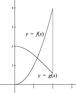
The figure below shows graphs of $y=f(x)$ and $y=g(x),\, 0\le x\le 2$ where $f(x)=1+\cos(x)$ and $g(x)=x^3$. Print two copies of the graphs.
| < Previous Section | Home | Next Section > |