Figure 8.4.5. $ds$ is an approximation of the arc length of $f$'s graph through this partial $\Delta x$-interval.
| < Previous Section | Home | Next Section>> |
In Section 8.3 we devloped methods for computing the volume of solids contained within a shell. In this section we will focus on quantifying the arc length of a graph and the surface area of a shell.
Our methods for computing arc length and surface area will resemble that for solids:
We approximated accumulated volume as we filled a shell with volumes of cylinders. We will approximate surface area of shells with surface area of cones (actually, parts of cones).
Figure 8.4.1 shows an outline of a football stadium being planned in a major city. The plan leads to project engineers needing to compute the arc length of a mathematical curve.
Figure 8.4.1.
Figure 8.4.2 tells the story of a city's beautification plan gone awry. The problem the plan created required project engineers to compute the area of a mathematical surface.
Figure 8.4.2. Unintended consequences of a city's beautification plan.
We will use calculus to build mathematical tools to address problems like those arising in Figures 8.4.1 and 8.4.2.
The idea of arc length of a function's graph over an interval is quite simple. Imagine covering the graph with a piece of string. Then stretch the string along the axis that holds the function's independent variable. The length of the string is the graph's arc length over that interval. Figure 8.4.3 illustrates this idea.
Figure 8.4.3. A graph's arc length over an interval is the length of string that covers the graph.
The arc length of the graph in Figure 8.4.3 over the interval $[0,4]$ is about 12.9 units.
While the idea of arc length is simple, it requires a bit of work to compute an arc length for a given function. The big idea is to accumulate the lengths of segments that approximate the graph over intervals of length $\Delta x$.
Figure 8.4.4 displays a graph of a function f. When you play the animation you see seven phases in conceptualizing a method for approximating the accumulated arc length of $f$'s graph as the value of x varies from -1.5 to 1.5.
Figure 8.4.4. Seven phases in conceptualizing accumulated arc length of $f$'s graph as the value of its independent variable varies over an interval.
The seven phases in Figure 8.4.4 unpack the idea of approximating arc length by using line segments that approximate the graph. The phases are:
To calculate arc length of a functions graph from $t=a$ to $t=x$ as the value of x varies, all we need is the rate at which accumulated arc length varies with respect to x.
Once we have the rate of change of arc length with respect to x, we calculate arc length over that interval by integrating the arc length's rate over that interval.
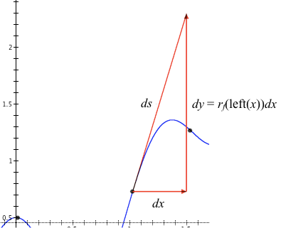
Figure 8.4.5 shows a frozen image of approximate arc length on the graph of $f$ while $dx$ varies through a $\Delta x$-interval.
Figure 8.4.5. $ds$ is an approximation of the arc length of $f$'s graph through this partial $\Delta x$-interval.
The value of $ds$ in relation to values of $dx$ and $dy$ can be derived using Pythagoras' Theorem: $$\begin{align} ds^2&=dx^2+dy^2\\[1ex] ds&=\sqrt{dx^2+dy^2}\\[1ex] ds&=\sqrt{dx^2+r_f(\mathrm{left}(x))^2 dx^2}\\[1ex] ds&=\sqrt{\left(1+\left(r_f(\mathrm{left}(x))\right)^2\right)dx^2}\\[1ex] ds&=\sqrt{1+\left(r_f(\mathrm{left}(x))\right)^2}dx\\[1ex] \frac{ds}{dx}&=\sqrt{1+\left(r_f(\mathrm{left}(x))\right)^2} \end{align}$$
For infinitesimal values of $\Delta x$,
Therefore, $r_s$, the exact rate of change of arc length of $f$'s graph with respect to its independent variable, is $r_s(x)=\sqrt{1+\left(r_f(x)\right)^2}$.
Reflection 8.4.1. How does the quotient of differentials $ds$ and $dx$ give an approximate rate of change of arc length of $f$'s graph with respect to x?
Reflection 8.4.2. Interpret the statement, "For infinitesimal values of $\Delta x$, $r_f(\mathrm{left}(x))$ is essentially equal to $r_f(x)$" in regard to Phase 7 of Figure 8.4.4.
Accumulated arc length on the graph of $f$ from $a$ to x is therefore $$\begin{align} \color{red}{\text{(Eq. 8.4.1)}}\qquad s_f(a,x)&=\int_a^x r_s(t)dt\\[1ex] &=\int_a^x \sqrt{1+\left(r_f(t)\right)^2}dt \end{align}$$
Figure 8.4.6 shows the graph of the function $h$ defined as $$h(x)=2\frac{\sin x}{x+1}e^{-\cos x}$$for $x \ge 0$.
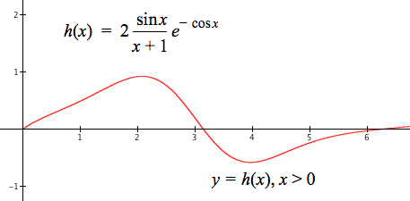
Figure 8.4.6. Graph of the function h for values of x greater than or equal to 0.
Our task is to define a function that gives the graph's arc length over any interval of its domain.
We know from above that the arc length of $h$'s graph over any interval $[a,x]$ is $s_h(a,x)=\int_a^x r_s(t) dt$, where $r_s(x)=\sqrt{1+\left(r_h(x)\right)^2}$. To define $s$ we therefore need to define $r_s$ and, by implication, $r_h$.
We can use GC's capabilities to define $h$'s arc length function $s_h$: $$\begin{align} s_h(a,x)&=\int_a^x r_s(t)dt\\[1ex] r_s(x)&=\sqrt{1+\left(r_h(x)\right)^2}\\[1ex] r_h(x)&=\frac{d}{dx}h(x) \end{align}$$
Figure 8.4.7 shows the graph of $y=s_h(a,x)$ as x varies from $a=1$.
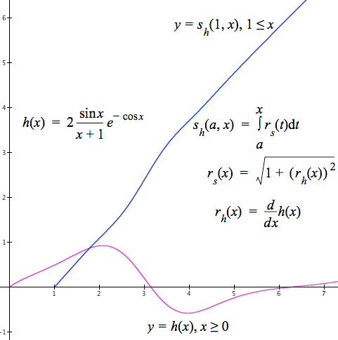
Figure 8.4.7.
Reflection 8.4.4.
Use GC to do the following for each of Exercises 1 through 4:
Function f defined as $f(x)=e^{\cos(x)}$. Interval: $x=2 \text{ to }x=5$
The idea of a shell's surface area is somewhat analogous to the idea of a graph's arc length.
The shell's surface area is the area of the region you would get if you could unwrap the shell and place it in a plane without distorting its surface. The area of the planar region is the surface area of the shell.
Figure 8.4.8 illustrates this idea with a right circular cone and a part of the cone (called a frustum).
Figure 8.4.8a. Unwapping a right circular cone into a plane figure without distorting the cone's surface.
Figure 8.4.8b. Unwapping a right circular frustum into a plane figure without distorting the frustum's surface.
Reflection 8.4.5. Be sure that you understand how a right circular cone unwraps into a sector of a circlular region and how a circular frustum (section of a cone) unwraps into a section of a circular region.
A right circular conic shell is one example of what is called a developable surface--a surface that can be unwrapped into a plane without distorting it. Developable surfaces can be quantified using geometry and algebra. Click here to see the derivation for surface area of a right cone. We will use this formula often, so please study it.
Figure 8.4.9 Shows three shells. Part (a), a right cone, is discussed above. Shells like these often can be treated with algebra and geometry to compute their surface areas.
Part (b), a paraboloid, is made by rotating $y=x^2$ around the y-axis. It is not a developable surface. You cannot unwrap it into a plane without distorting the surface. We will use the calculus you now know to compute surface areas of shells like this.
Part (c) is called Boy's Surface. Boy's Surface also is not developable. Defining Boy's Surface and computing its area requires function definitions and integration techniques that you will learn in Calculus III.
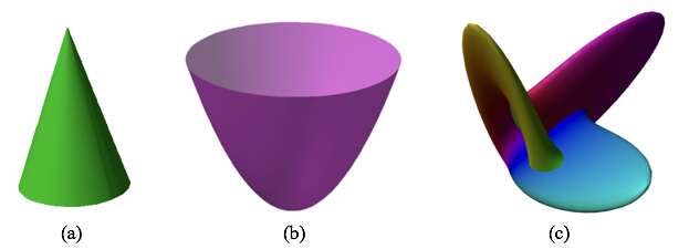
Figure 8.4.9. Three surfaces: (a) A circular cone, (b) a paraboloid, and (c) Boy's Surface.
We will follow the general theme that to define an accumulation function $S$ (in this case, accumulating surface area) we integrate the accumulation's rate of change function $r_S$ over an interval whose length varies with the function's independent variable.
We therefore need to come up with a function $r_S$ whose values $r_S(x)$ give the rate of change of accumulating surface area as the function's independent variable x varies.
Once we have $r_S$, we can define $S$ as$$S(a,x)=\int_a^x r_S(t)dt$$
Figure 8.4.10 shows a surface created by revolving a graph around the x-axis. When you play the animation you see the surface being covered by sections of cones (called frusta, plural of frustum).
Figure 8.4.10. A shell's surface area approximated by conical frusta. The first pass shows frusta graphed as the value of x varies by $dx$ through large $\Delta x$-intervals. The next two show frusta as x varies by $dx$ through smaller $\Delta x$-intervals.
Figure 8.4.11 isolates the frustum that is growing in slant height as x varies by $dx$. Please understand that we show a visually large value of $ds$ as an aid to understanding the following discussion. But the discussion speaks of $ds$ as varying thorugh $\Delta x$-intervals of infinitisemal size.
Figure 8.4.11 focuses on three things:
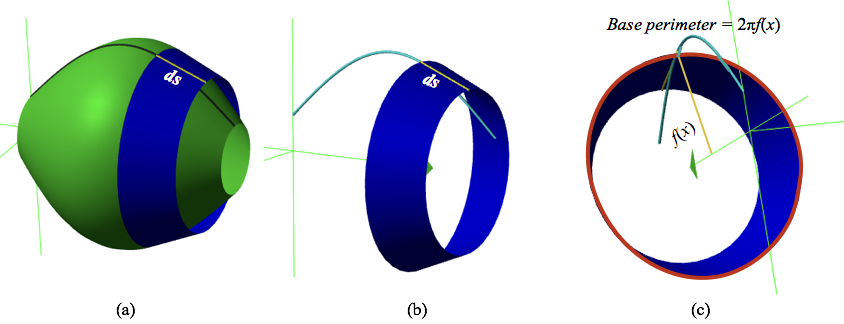
Figure 8.4.11.
Figure 8.4.12 unwraps the frustum to make it easier to see the rate at which the frustum's area varies as $ds$ varies.
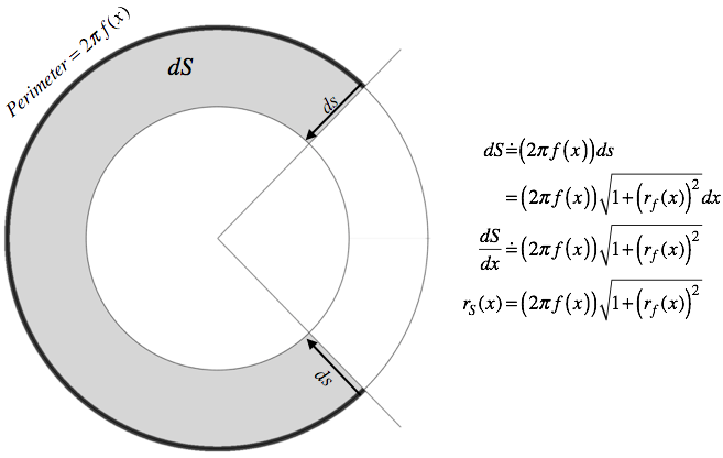
Figure 8.4.12. The frustum unwapped into a circular segment.
$ds$ is the approximation to the function's accumulated arc length over the current $\Delta x$-interval.
It is important to understand the role played by $ds$, the approximate arc length of $f$'s graph as x varies by $dx$, and $2\pi f(x)$, the frustum's base perimeter. Look back and forth at Figures 8.4.11 and 8.4.12:
Reflection 8.4.6. Print Figure 8.4.12. Cut out the shaded region (including the statement "$Perimeter=2\pi f(x)$"). Pull the ends of the region you cut out together. You will form a frustum with slant height $ds$ and base perimter $2\pi f(x)$. Compare your frustum to Figure 8.4.11, part (c).
We can now complete our plan for computing surface area of a shell of revolution.
We started by creating a shell by rotating the graph of a function $f$ around an axis. We thought of the shell's surface area as accumulating as the function's independent variable varies, creating an accumulation function $S$ whose value $S(a,x)$ gives accumulated surface area from $a$ to x.
We wanted to end with a function $S(a,x)=\int_a^x r_S(t)dt$, where $r_S(x)$ is the exact rate of change function for $S$.
To define the surface area function S, we needed to define $r_S$, the function that give the exact rate of change of a shell's surface area with respect to the function's independent variable. We defined $r_S$ as $$r_S(x)=2\pi f(x)\sqrt{1+\left(r_f(x)\right)^2}$$
We can now define the surface area function S as $$\begin{align}\color{red}{\text{(Eq. 8.4.2)}}\qquad S(a,x)&=\int_a^x r_S(t)dt\\[1ex] &=\int_a^x 2\pi f(t)\sqrt{1+\left(r_f(t)\right)^2}dt \end{align}$$
Figure 8.4.14 shows the graph of $y=f(x)$ where $f(x)=0.5+\dfrac{x}{\sqrt{x+1}}+0.1\sin(10x)$.
Figure 8.4.15 shows the shell generated by rotating the graph of $f$ over the interval $[0,2]$ around the x-axis and the approximate accumulated surface area as x varies by $dx$ through $\Delta x$-intervals of length 0.01.
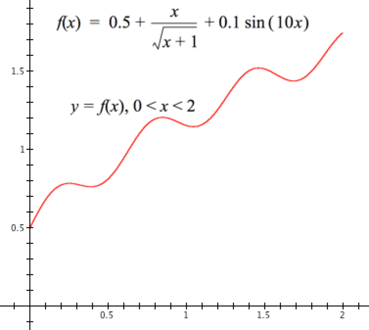
Figure 8.4.14.
Figure 8.4.15.
Figure 8.4.16 shows a GC file that applies the definition of $S$ given in Eq. 8.4.2 to the problem of modeling this surface area..
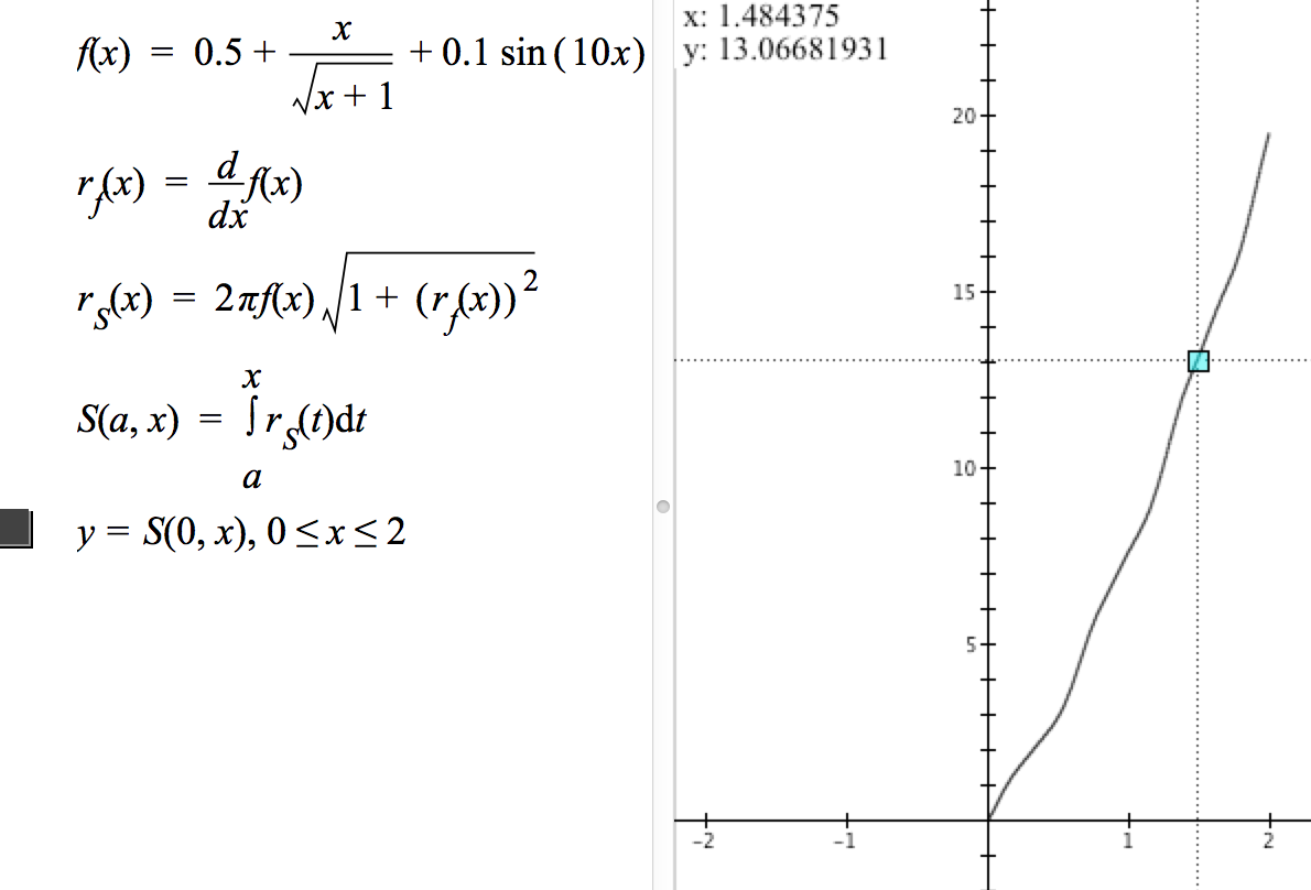
Figure 8.4.16.
The following reflections are all in relation to Figure 8.4.16.
Reflection 8.4.7. A point is highlighted on the graph of $y=S(0,x)$. Its coordinates show in the upper left corner of the graph pane. What does each number mean?
Reflection 8.4.8. How does the second line define $r_f(x)$ so that GC can evaluate $r_f(1.3)$?
Reflection 8.4.9. In GC, type the function definitions in Figure 8.4.16. Re-define $r_f$ so that it is defined explicitly, in closed form. Do you get the same graph for $y=S(0,x)$?
Each function in Exercises 1-4 is defined over an interval I. Assume that independent variables are measures in meters.
Consider the surface that is generated by revolving the function's graph over that interval around the indicated axis. Do the following for each function.
$f(x)=3+\sqrt{0.5+x}$ rotated around the x-axis, $0\le x\le 4$. What is $S(1, 1.5)$? What does this number mean?
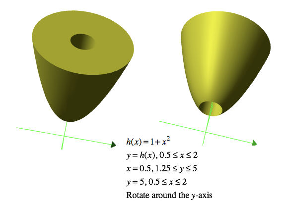
Let $h(x)=1+x^2$. Rotate $$\begin{align}y&=h(x),\, 0.5\le x\le 2\\[1ex]x&=0.5,\,1.25\le y\le 5\\[1ex]y&=5,\, 0.5\le x\le 2\end{align}$$ around the y-axis. (See below.) Be sure to include surface area of the inner tube and accumulated surface area on the top as your accumulated surface area's independent variable varies.
What is the surface area of the entire shell?
(Adapted from Briggs &Cochran, Exercise 6.6.35)
The ratio of an object's surface area to its volume (SAV) is important in animal biology.
Animals typically generate heat at a rate that is proportional to their volume and lose heat at a rate that is proportional to their surface area.
Therefore, animals with a low SAV ratio (such as elephants) tend to retain heat, whereas animals with a high SAV ratio (such as children) lose heat relatively quickly.
| < Previous Section | Home | Next Section>> |