Figure 8.5.1. GC's graphs of the rate of change functions for Disease A and Disease B.
| < Previous Section | Home | Next Section > |
It is common for people to think of the physical and social sciences as being in intellectual opposition. They think of the physical sciences as being about inanimate natural objects while thinking of the social sciences as being about interactions among living beings.
However, when you think of quantities varying at some rate with respect to each other, then the ideas of calculus apply whether the quantities are numbers of people having certain characteristics at various moments in time or the force of gravity acting on an object at different distances from Earth's surface.
If you can state a relationship between variations in quantities' values, then the ideas of calculus will apply.
It is imperative that you use GC to follow the examples in this section.
Disease A and Disease B spread at different rates.
Disease A spreads slowly at first and more rapidly as time passes.
Disease B spreads rapidly at first and less rapidly as time passes.
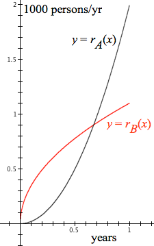
Disease A spreads at a rate of $$r_A(t)=2000t^2\qquad \text{persons/year}$$for each value of t in the first year.
Disease B spreads at a rate of $$r_B(t)=1100\sqrt t\qquad \text{persons/year}$$for each value of t in the first year.
Figure 8.5.1 shows GC's graphs of the diseases' rate of change functions.
Figure 8.5.1. GC's graphs of the rate of change functions for Disease
A and Disease B.
Question: Which disease infects the most people in the first year?
It seems intuitive that Disease A will infect more people in the first year because its rate of infection becomes so much greater than that of Disease B.
Now we'll take a closer look.
At any moment t, Disease A spreads at the rate of $r_A(t)$ persons/year. The number of people infected by Disease A over a small interval of time $dt$ (e.g., 0.01 years) at any value of t is essentially $r_A(t)dt$.
So the number of people in total who have been infected by Disease A from the beginning of the year up to t years will be the accumulation of those incremental variations as time varies from $u=0$ to $u=t$, or $$A(t)=\int_0^t r_A(u)du.$$
Similarly, at any moment t, Disease B spreads at the rate of $r_B(t)$ persons/year. The number of people infected by Disease B over a small interval of time $dt$ (e.g., 0.01 years) at any value of t is essentially $r_B(t)dt$.
The number of people in total who have been infected by Disease B from the beginning of the year up to t years will be the accumulation of those incremental variations as time varies from $u=0$ to $u=t$, or $$B(t)=\int_0^t r_B(u)du.$$
Figure 8.5.2 shows the graphs of $y=A(x)$ and $y=B(x)$ for $0 \le x \le 1$. We can see that Disease B has infected more people at all moments in time during the first year despite the fact that, as we saw in Figure 8.5.1, Disease A's rate of change is much larger than Disease B's rate of change for most of the latter half of the year.
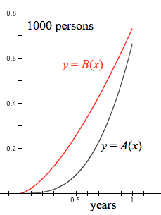
Figure 8.5.2. GC's display of the graphs of $y=A(x)$ and $y=B(x)$.
Enter definitions of $r_A,\, r_B,\, A,\, \text{ and }B$ into GC, and evaluate $A(1)$ and $B(1)$. You will see that, according to these models, at the end of the first year approximately 667 people were infected by Disease A and approximately 733 people were infected by Disease B.
Toy cars 1 and 2 start simultaneously from the same starting line. Car 1 accelerates rapidly early in the race and less rapidly later. Car 2 accelerates slowly at the beginning of the race and then rapidly later.
Car 1 accelerates at each moment of t at the rate of $$a_1(t)=0.7t+\sin\left(\dfrac{3\pi t}{5}\right)\text{ (ft/sec)/sec.}$$
Car 2 accelerates at each moment of t at the rate of $$a_2(t)=3-3\cos\left(\dfrac{2\pi t}{15}\right)\text{ (ft/sec)/sec.}$$
What are the car's relative speeds at each moment in time? Which car is going faster at the end of 8 seconds?
What are the car's relative distances at each moment in time? Which car has gone farther at the end of 8 seconds?
Figure 8.5.3 shows GC's display of graphs for Car 1's and Car 2's acceleration functions with respect to elapsed time. Car 1 accelerates more rapidly than Car 2 in the first part of their race, Car 2 accelerates more rapidly in the second part of their race, and so on.
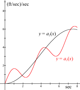
Figure 8.5.3. GC's display of the acceleration functions for Car 1 and
Car 2.
If we think carefully about Figure 8.5.3 in terms of what is happening to cars' velocities, then we can see that since Car 1 starts with higher accelerations, it will have greater velocity than Car 2.
Even when the cars have equal accelerations at about $t=1.9$ seconds, Car 1 will have a higher velocity. So it will take some time after the cars first have equal accelerations that their velocities will be the same.
However, we cannot tell when. Also, it is not clear from these graphs which car is ahead at the ends of the second, third, and fourth parts of their race.
We need to see their velocities at each moment in time.
Acceleration is a rate of change of velocity with respect to time. To derive velocity from acceleration, we note that at any moment t, a car is accelerating at $a(t)$ (ft/sec)/sec over a tiny interval of length $dt$ seconds, so at t seconds a car's velocity will vary by $a(t)dt$ ft/sec.
Let values of the function $v_1$ at a value of t be the accumulated velocity $v_1(t)$ of Car 1 after t seconds have elapsed. Values of $v_1$ will therefore be $${\displaystyle v_1(t)=\int_0^t a_1(u)du}.$$
Let values of the function $v_2$ at a value of t be the accumulated velocity $v_2(t)$ of Car 2 after t seconds have elapsed. Values of $v_2$ will therefore be $${\displaystyle v_2(t)=\int_0^t a_2(u)du}.$$
Figure 8.5.4 shows GC's graphs of $y=v_1(x)$ and $y=v_2(x)$. As elapsed time increases, Car 1 goes at a higher velocity than Car 2, then Car 2 goes at a higher velocity than Car 1. The graphs in Figure 8.5.4 allow us to answer the question of which car is going faster at the end of 8 seconds. Car 2 is going faster.
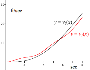
Figure 8.5.4. GC's display of the velocity graphs $y=v_A(x)$ and
$y=v_B(x)$.
You can find out how fast each car is going after 8 seconds have elapsed.
Reflection 8.5.0 Compare Figures 8.5.3 and 8.5.4 in terms of when the cars have equal accelerations and when they have equal velocities.
We still have not determined which car is ahead after 8 seconds have elapsed. We need to see their distances traveled at each moment in time.
Velocity is a rate of change of displacement with respect to time. Since the cars move in one direction, displacement and distance are the same thing. To derive distance from velocity, we note that at any moment t, a car is traveling at $v(t)$ ft/sec over a tiny interval of length $dt$ seconds, so at t seconds a car's distance will vary by $v(t)dt$ ft.
Let values of the function $s_1$ at a value of t be the accumulated distance $s_1(t)$ after t seconds have elapsed. Values of $s_1$ will therefore be $${\displaystyle s_1(t)=\int_0^t v_1(u)du}.$$
Let values of the function $s_2$ at a value of t be the accumulated distance $s_2(t)$ after t seconds have elapsed. Values of $s_2$ will therefore be $${\displaystyle s_2(t)=\int_0^t v_2(u)du}.$$
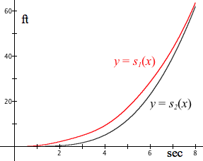
Figure 8.5.5 shows GC's display of the graphs of $y=s_1(x)$ and $y=s_2(x)$. Surprisingly, after they start, Car 1 is ahead of Car 2 throughout the race despite Car 2 going faster than Car 1 at the end of the race.
Study Figures 8.5.3, 8.5.4, and 8.5.5 in terms of what each represents (acceleration at a moment, velocity at a moment, distance at a moment) so that it makes sense to you that, once they start, Car 1 is always ahead of Car 2.
You should have entered all the function definitions for Example 2 and generated all the graphs in Figures 8.5.3, 8.5.4, and 8.5.5 as you followed the discussions. If you did not do this, then do it now.
Figure 8.5.6 repeats what you saw (assuming you did) when graphing $y=s_1(x)$ and $y=s_2(x)$. It shows that GC takes a long time to display these graphs. Why?
Think about why GC takes so long to generate these graphs before reading on.
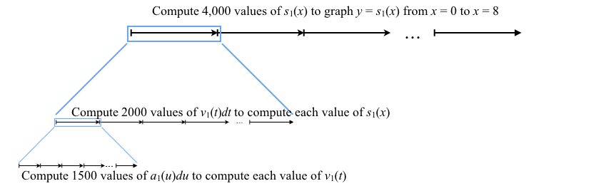
For GC to calculate a value of, say, $s_1(4.1)$ it must calculate bits of distance $v_1(t)dt$ for many values of t from 0 to 4.1.
But to calculate a value of $v_1(t)dt$ for any value of t, GC must also calculate many values of $a_1(u)du$ for values of $u$ ranging from 0 to t.
To display the graph of $y=s_1(x)$ GC must repeat this double-variation process for all (actually, a large sample) of values of x from $x=0$ to $x=8$.
Figure 8.5.7 illustrates the above explanation graphically.
Suppose that:
GC does an enormous number of computations to compute values of $s_1$ and $s_2$. This is why it takes so long to generate the graphs in Figure 8.5.6.
We could dramatically reduce the number of computations GC must do to compute values of $s_1$ and $s_2$ by defining them in closed form. Producing closed form definitions of accumulation functions defined in open form will be the focus of Chapter 9.
We will remind you in Chapter 9 of this digression as motivation to find closed form definitions of accumulation functions. In this chapter, we use integral functions defined in open form to focus on uses of calculus to conceptualize quantitative situations.
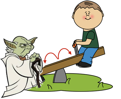
Yoda and Little Lukey are on opposite ends of a seesaw (Figure 8.5.8). Yoda's mass is 81.8 kg. Lukey's mass is 54.5 kg. Lukey sits 1.8 meters from the seesaw's center. The seesaw balances when no one sits on it. How far from the seesaw's center must Yoda sit so that he and Lukey balance each other?
The physics of a seesaw entails two opposing rotational (twisting) forces. The measure of a rotational force is called torque. So Yoda and Lukey will balance each other when the torques on either side of the seesaw have equal magnitudes and opposite rotational directions.
Figure 8.5.9 presents the standard image for torque as a force applied perpendicularly to an object that rotates around a pivot point (fulcrum).
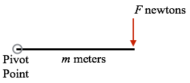
Figure 8.5.9. A force of F Newtons applied at a distance of m meters
from a pivot point
(fulcrum) creates a torque of $F\cdot m$ Newton-meters.
Torque is calculated as $force\cdot distance$. The SI unit for torque is the Newton-meter, or N-m, which is a rotational force of 1 Newton acting at a distance of 1 meter from a fulcrum. One Newton of force is the force that accelerates a mass of 1 kg at a rate of 1 (m/s)/s.
Lukey's weight is a force pushing down on Lukey's end of the seesaw. Yoda's weight is a force pushing down on Yoda's end of the seesaw. Weight at Earth's surface is the force due to a mass being accelerated by gravity. Acceleration due to gravity at Earth's surface, in the SI system, is $9.8 \mathrm{\frac{(m/s)}{s}}$ (taking down as positive).
Lukey's force on the seesaw when it is in balance will therefore be $9.8\,\mathrm{\dfrac{(m/s)}{s}} \cdot 54.5 \text{ kg}$, or 534.10 Newtons. Yoda's force on the seesaw when it is in balance will be 801.64 Newtons.
For Yoda and Lukey to balance on the seesaw they must exert torques that are equal in magnitude but opposite in direction. Lukey's torque will be $534.10 \cdot 1.8$ N-m, or 961.38 N-m when he and Yoda are in balance. Yoda will sit $k$ meters from the fulcrum and exert a torque of $-(801.64 \cdot k)$ N-m when he and Lukey are in balance.
For the seesaw to balance, $$\begin{align}-(801.64\cdot k)&=961.38\\[1ex] k&=\frac{961.38}{-801.64}\\[1ex] &\approx -1.20\end{align}$$So, for the seesaw to balance, Yoda must sit approximately -1.20 meters from the fulcrum, or 1.20 meters on the opposite side of the fulcrum from Lukey when Lukey sits 1.8 meters from the fulcrum.
A beam is 0.05 m high, 0.1 m wide, 2.5 m long, and has uniform vertical density but a horizontal density that varies with distance from its fulcrum (Figure 8.5.10).

The beam's density is 2200 $\mathrm{kg/m^3}$ at the fulcrum, 5400 $\mathrm{kg/m^3}$ at the other end, and varies linearly from fulcrum to end. What torque does any portion of the beam exert at the fulcrum?
That is, suppose you cut the beam x meters from the fulcrum. What torque would the beam of length x exert at the fulcrum?
Example 3 is just like the seesaw when we think of a small slice of the beam exerting, by itself, a rotational force.
Figure 8.5.11a illustrates conceptualizing accumulated torque as the beam's length varies.
Figure 8.5.11a. Imagine the beam's length varying by dx through intervals of size $\Delta x$ and having constant density within $\Delta x$-intervals.
It will be important to note that variations in the volume of a slice that is 0.05 m wide, 0.1 m high, and has a thickness of $dx$ m will be $dV=Adx \mathrm{\,m^3}$, where $A=0.05\cdot 0.1$ (see Figure 8.5.11b).
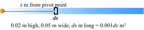
Figure 8.5.11b. Side view of a slice of length dx has a volume of 0.001dx$\text{ m$^3$}$ as the value of x varies by dx through an interval of size $\Delta x$.
Imagine the beam varying in length from the fulcrum along the beam's axis as in Figure 8.5.11a. Let x be the beam's length from the fulcrum as the length increases.
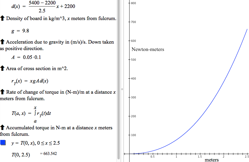
As x varies from 0 to 2.5, the beam's density varies from 2200 $\mathrm{kg/m^3}$ to 5400 $\mathrm{kg/m^3}$. The beam's density (rate of change of mass with respect to volume) at a distance of x m from the fulcrum is therefore given by the function $d$ defined as $$d(x)=\frac{5400-2200}{2.5}x+2200 \mathrm{\quad kg/m^3}.$$Remember that density is a rate of change of mass with respect to volume, and that the volume of a cylinder varies at a rate that has the same numerical value as its base.
Figure 8.5.12 shows GC's display of a graph of the torque exerted by the part of the beam from 0 meters to x meters along the beam as x varies from 0 to 2.5. The torque exerted by the entire beam is $T(0,2.5)\approx 663.54$ Newton-meters. Click here to download the GC file.
Reflection 8.5.1. What would be the the beam's total torque at its fulcrum were everything to stay the same except its height and width:
Population growth rates are expressed in terms of a percent of the current number of persons in the population by which the population increases per year. The U.S. population grew approximately 0.77% from July 1, 2015 to July 1, 2016. If we let P be the function that gives the U.S. population in relation to number of years CE, then $P(2016.5)=1.0077P(2015.5)$.
Let t be number of years since July 1, 2016. Let $P_0$ be the U.S. population on July 1, 2016. What, approximately, will be the U.S. population at each moment in time after July 1, 2016 if the population continues to grow at an annual rate of 0.77% per year?
If the U.S. population were to continue growing continuously by 0.77% per year, then its rate of growth in number of people per year would be $r_P(t)=0.0077P(t)$, or in prime notation, $P'(t)=0.0077P(t)$. This says that the rate of change of a population in persons/year at any moment is proportional to the number of people in the population at that moment.
We saw in Chapter 6 that the exponential function is the only function that has a rate of change at a moment that is proportional to its value at that moment. $P$ is therefore an exponential function.
Put another way, $e^{kt+c}$ is an antiderivative of $ke^{kt+c}$ (you should check this). Thus, $r_P(t)=kP(t)$ implies that $$\begin{align}P(t)&=\int_0^t ke^{ku+c}du\\[1ex]
&=e^{kt+c}\\[1ex]
&=e^c \cdot e^{kt}.\end{align}$$
At $t=0$, $P(0)$ is the population on July 1, 2016, so $P(0)=P_0$. But $$\begin{align}P(0)&=e^c\cdot e^{k\cdot 0}\\[1ex]&=e^c\end{align}.$$Hence $P_0=e^c$, and therefore $$\begin{align}P(t)&=e^ce^{0.0077t}\\[1ex]&=P_0e^{0.0077t}\end{align}.$$
We hasten to point out that, in the case of exponential growth, we were unable to represent the accumulation function as an open form integral. We needed to make the connection that exponential functions are the only functions that have a rate of change at a moment that is proportional to the value of the function at that moment.
This connection, between exponential functions and rate of change being proportional to the value of the function, will be key in many applications.
Population ecologists study the dynamics of species populations and how they interact with their environments, especialy how population sizes vary over time and space.
Ecologists use mark and recapture techniques to estimate the population of a species. When they do this two years in a row they can estimate the population's annual growth rate.
A population's environment constrains its size. As the population grows, resources become insufficient to support continued growth, and growth slows until the population reaches its maximum sustainable size.
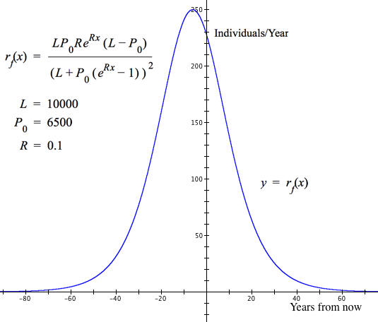
Ecologists developed a model for the rate of change of population size in constrained environments. The function $r_P$ defined below takes into consideration the population's maximum sustainable size $L$, the current populaton size $P_0$ and the natural growth rate $R$ when the population is sufficiently small that it is not stressing its environment.
$$r_P(x)=\frac{LP_0Re^{Rx}(L-P_0)}{\left(L+P_0\left(e^{Rx}-1\right)\right)^2}$$
Any function P that has a rate of change function $r_P$ of this form is called a logistic growth function, and $r_P$ is called a logistic rate of change function.
Figure 8.5.15 shows GC's graph of $y=r_P(x)$ for $L=10,000$, $P_0=6,500$, and $R=0.1$ (growth rate of 10% per year), and $x=\text{ number of years from a reference year}$.
Population growth with respect to time typically fits the logistic model when the population is constrained to an environment that has a limited capacity to support it.
The logistic rate function $r_P$ gives the rate of change of the population function $P$ at all moments since the reference year.
We can therefore define the function $P$ so that $P(x)$ gives the population at any mumber of years from the reference year. We do this by adding the net variation in population from the reference year to the population at the reference year.
Net variation in the population x years away is made by accumulating bits of variation $r_f(t)dt$ as t varies from $t=0$ to $t=x$. We therefore define $P$ as$$P(x)=P_0+\int_0^x r_P(t)\,dt$$Figure 8.5.16 shows the graph of $y=P(x)$ with the $r_P,\,P_0,\,L,\,\text{ and }R$ defined as in Figure 8.5.15.
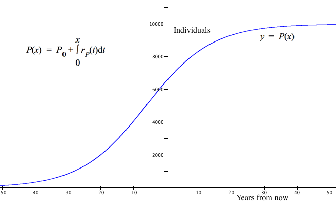
Notice that the graph of $y=P(x)$ shows the value of $P(x)$ is $P_0=6,500$ at $x=0$, and the value of $P(x)$ approaches $L=10,000$ as the number of years from the reference year increases.
Pierre Verhulst introduced the idea of a logistic function in his attempt to model population growth in constrained environments. As we will see in the exercises, the logistic function shows up in many contexts other than population growth.
Reflection 8.5.1x. The graph of $y=P(x)$ shows values of $P(x)$ for negative values of x. The value of $P(-10)$ is approximately $4059$. What does $-10$ mean? What does $4059$ mean? How does the definition of P work so that $P(-10)\approx 4059$?
A herd of deer lives in a valley that isolates them from other herds. Population ecologists estimate that the valley's resources can support a maximum population of 6,000 deer. The ecologists used a mark and recapture method to estimate the current population to be 1500 deer. The ecologists infer from past samplings that the population has a natural growth rate of approximately 8%/yr.
Park managers want to limit the population to 5000 deer to keep the population safe from disease and deprivation. They will do this by issuing hunting licenses when the population reaches 5000 deer.
Use the logistic function $P$ and the logistic rate function $r_P$ to estimate when they must start limiting the population and the number of hunting licenses they should plan to issue each year.
The park managers will use the functions $P$ and $r_P$ with $L=5000,\ P_0=1500,\, \text{ and }R=0.08$. Figure 8.5.16-2 (note to self--renumber figures) shows the graph of $y=P(x)$ with these parameter values and $r_P$ defined as in Figure 8.5.15.
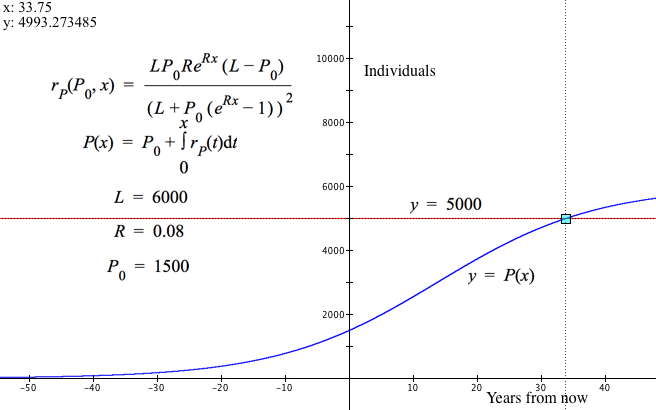
Figure 8.5.16-2. Population graph for this deer herd (with parameters as shown), and the graph of $y=5000$. The graphs intersect at $x\approx 33.8$ and $P(x)\approx 5000$.
The graphs of $y=P(x)$ and $y=5000$ intersect at $x\approx 33.8$ years from the moment of making their model. So they should plan on issueing hunting licenses in 34 years.
GC reports $r_P(34)\approx 66.14$, which means that the population 34 years from now will vary by approximately 66 deer per year if nothing is done. So park managers can plan to issue 66 hunting licenses per year starting in 34 years. Of course, they will continue to monitor the deer population periodically and adjust accordingly. But this is their plan as of now.
Reflection 8.5.1y. The park managers would like to define a function Q whose values will give the net variation in population between any two values of x. Define Q for them.
We know from experience that consuming alcohol dulls our senses and affects our moods. We can use calculus to model alcohol's effect over time.
Blood alcohol concentration (BAC) is measured in milliliters of alcohol per liter of blood. According to this website, different BAC levels produce these effects:
| Euphoria | BAC 0.03 to 0.12 |
| Excitement | BAC 0.09 to 0.25 |
| Confusion | BAC 0.18 to 0.30 |
| Stupor | BAC 0.25 to 0.40 |
| Coma | BAC 0.35 to 0.50 |
| Death | BAC > 0.50 |
In most states in the U.S., a BAC of 0.05 or greater is cause for a combination of arrest, imprisonment, loss of drivers license, confiscation of your car, or high fine.
One 12-ounce glass of beer, one 5-oz glass of wine, and one 1.5-oz shot of whiskey typically contain 18 milliliters of alcohol. We will call each of these "a drink". So, a drink in any of these forms contains 18 ml of alcohol.
Ron is at a party. He weighs 198 lbs (90 kg). He chugs (consumes rapidly) 3 drinks, 15 minutes apart. What is Ron's BAC over time?
When you consume alcohol, it is simultaneously absorbed into your bloodstream and eliminated by your liver.
Alcohol is absorbed into your bloodstream at a rate (in milliliters of alcohol per liter of blood per hour since consumption) that is proportional to the amount of alcohol that is available to absorb.
Your liver eliminates alcohol from your bloodstream at a rate (in milliliters of alcohol per liter of blood per hour since consumption) that is proportional to the amount of alcohol in your bloodstream.
The rate at which a person's BAC varies with respect to time is the difference between the rate at which alcohol is absorbed and the rate at which it is eliminated.
The rate at which a person's BAC variations in (ml/liter)/hr is also affected by his or her mass and the amount of alcohol consumed.
When a person with mass $M$ kg consumes $V$ ml of alcohol, the rate at which his or her BAC varies with respect to the number of hours since consuming it is modeled (approximated) by the function $r_B$, defined asRon drank his first drink at $t=0$ hours. He drank his second drink at $t=0.25$ hours. He drank his third drink at $t=0.5$ hours. The rate at which Ron's BAC varies over time is therefore
$$r(t)=r_B(t)+r_B(t-0.25)+r_B(t-0.50).$$
Reflection 8.5.2. Explain how $r_B(t-0.25)$ gives the rate at which Ron's BAC varies that is due to the $2^{nd}$ drink and how $r_B(t-0.50)$ gives the rate at which Ron's BAC varies that is due to the $3^{rd}$ drink. Then explain how the sum $r_B(t)+r_B(t-0.25)+r_B(t-0.50)$ gives the rate of change of Ron's BAC at all moments of t, $0 \le t$.
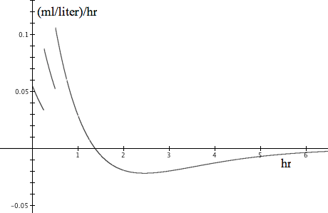
Figure 8.5.17 shows GC's display of the rate at which Ron's BAC varies with respect to time at each moment since consuming his first drink. Discontinuities in the graph are because we assumed that Ron consumed each drink instantaneously, which of course is impossible, but is nevertheless a useful assumption to simplify our model. This is an instance of George Box's famous aphorism, "all models are wrong, but some are useful".
Reflection 8.5.3. Elaborate
on the comment that discontinuities in the graph in Figure 8.5.17 are
due to the assumption that Ron consumed each drink instantaneously.
Reflection 8.5.4. Explain how the graph in Figure 8.5.17 makes sense in relation to Ron's consumption and the way that alcohol is absorbed and eliminated from the bloodstream. Think especially about why the rate jumps when it does, and what it means for values of $r_B(t)$ to be positive or negative.
According to our model, each value $r(t)$ is the exact rate of change of Ron's BAC at each moment of t. So Ron's BAC will vary by $r_B(t)\,dt$ as $dt$ varies through moments in time.
Ron's BAC over time will be the accumulation of variations in his BAC. The function $B_3$ (BAC after 3 drinks), defined as $$B_3(t)=\int_0^t r(u)du$$ will, according to our model, give Ron's BAC from $u=0$ to $u=t$ hours since consuming his first drink when he consumes 3 drinks 0.25 hours apart.
Figure 8.5.18 shows GC's display of $y=B_3(x)$, which is a model of Ron's BAC over time. His BAC becomes illegal approximately 0.75 hours after his first drink and does not return to a legal level until approximately 2.3 hours after his first drink.
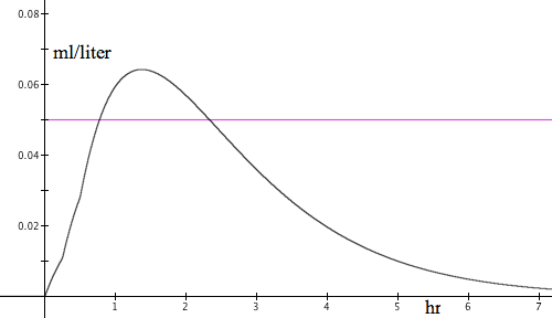
Figure 8.5.18. Ron's BAC over time since consuming his first drink and
consuming 3 drinks 0.25 hours apart.
Reflection 8.5.5. Explain how the graph in Figure 8.5.18 makes sense in relation to the rate at which Ron's BAC varies with respect to time as shown in Figure 8.5.17.
The common meaning of "work" is to make something happen by physical exertion. The technical notion of work is related to the common notion, but it is stated in a way that we can quantify it.
The physical quantity work (also called mechanical, or accomplished work) is defined to be a force applied over a distance.
In the SI system, force is measured in Newtons [the force required to accelerate a mass of 1 kg at a rate of 1 (m/s)/s] and distance is measured in meters.
The unit of mechanical work is called a joule, or the work accomplished by a force of 1 Newton applied constantly on an object through a displacement of 1 meter. So one joule is one N-m.
Reflection 8.5.6 Notice that time is not involved in the definition of work. It does not matter whether it takes 10 sec or 10 years to move an object a distance of 1 meter with a force of 1 Newton. The accomplished work either way is 1 joule, or 1 N-m.
The work accomplished to accelerate a 2 kg mass at a rate of 3 (m/s)/s over a distance of 5 meters is 30 joules. The net force applied to the object over this 5 meters was $2\cdot 3$ kg-(m/s)/s, or 6 Newtons. So the accomplished work was $2\cdot 3\cdot 5$ N-m, or 30 joules.
Notice that we did not know the object's initial velocity. If initial velocity was high, it took little time. If initial velocity was small, it took more time.
But the amount of time required to move the object 5 meters does not matter. A constant force of 6 Newtons was applied over a distance of 5 meters, which produced 30 joules of work.
The above example is of accomplished work after an object is displaced 5 meters. However, we can think of work as accumulating while an object is displaced.
We would then have accomplished work defined as an accumulation function, one that gives accomplished work at each distance that the object is displaced.
In the case of a constant force of $F$ Newtons applied over a distance of x meters, accomplished work as the value of x varies is $W=Fx$.
This implies that $dW=F\,dx$, which then implies that the constant force $F$, applied as $dx$ varies through an interval of length $\Delta x$, is the rate of change of accomplished work with respect to displacement.
In the case of variable force, where $F$ varies with displacement x, the differential in work $dW$ is $dW=F(x)dx$ as $dx$ varies over displacements of infinitesimal length.
Stated symbolically in three notational systems,$$\begin{align} r_W(x)&=F(x)\text{, where $F(x)$ is the force being applied at a displacement of $x$ meters}\\[1ex] \frac{dW}{dx}&=F(x)\\[1ex] W'(x)&=F(x) \end{align}$$
The accumulation function for accomplished work over a displacement from $t=a$ to $t=x$ is therefore,$$W(a,x)=\int_a^x F(t)dt$$
A winch lifts a platform from the ground to the top of a building by a thick cable. The rate of change of cable weight is 151.77 N/m. The platform structure (including people) weighs 2815 N. The winch must lift the floor of the platform 93 m for people to step onto the building's top.
Define a function $W$ whose values $W(h)$ give the accumulated work at each height $h$ above the ground as $h$ varies from 0 to 93.
The platform's weight is constant. It will not vary as the platform rises. Therefore, the work to raise just the platform $h$ meters will be the platform's weight times the height it is raised, or $2815h$ joules. The work to raise the platform from a height of $a$ meters to a height of $h$ meters is $2815(h-a)$ joules.
The weight of the cable (i.e., the force of gravity on the cable) between the winch and platform, however, will vary as the platform rises.
Reflection 8.5.7. Could we have defined $r_W$ as $r_W(h)=2815+151.77(93-h)$ and W as $\displaystyle{W(a,h)=\int_a^h r_W(t)dt}$? What would $r_W$ mean when defined this way?
Figure 8.5.19 shows GC's display of the graph of accomplished work at each height to which the platform is lifted.
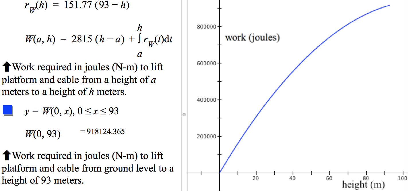
Figure 8.5.19. The graph of $y=W(x)$ as x varies from 0 to 93.
Reflection 8.5.8. In the platform scenario, the work we calculated assumed that the force applied by the winch counter-balanced the combined weights of the platform and cable.
However, to lift the platform and cable the winch must apply a force that exceeds these weights. An excess force at each height will determine the rate at which the platform and cable rise with respect to time.
Some springs, like a screen door spring, are designed to stretch and retract. Other springs, like an automobile's suspension spring, are designed to compress and expand.
Hooke's Law states that, within a range that depends on the spring, the force required to keep a spring in an expanded or compressed state is proportional to the spring's displacement from rest (Figure 8.5.20). The constant of proportionality is a measure of the springs stiffness.
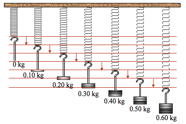
Figure 8.5.20. The force required to maintain a spring in its current (stretched or compressed) state is proportional to the spring's displacement from its natural resting state.
Hooke's law is expressed symbolically as $F(x)=kx$, where $F(x)$ is in Newtons, x is in meters, and $k$ is a measure of the spring's stiffness in Newtons/meter.
$dW$, the work required to stretch the string from any state by $dx$ as $dx$ varies infinitesimally, is $dW=F(x)dx$. $F(x)$ is therefore the rate of change of work accomplished when stretching the string when it is already stretched x meters from its resting state.
Suppose a spring stretches 0.03 m when a mass of 1.2 kg is hung from it. How much work would it require to stretch the string x meters, $0\le x \le 1$?
We need to first determine the spring's stiffness. A mass of 1.2 kg exerts a force due to gravity of $9.8\cdot 1.2=11.76$ Newtons. This force stretches the spring 0.03 meters. The spring's stiffness is $11.76/0.03=392$ N/m.
The force required to hold the spring at a displacement of x meters is $F(x)=392x$ N.
As in all cases of mechanical work, the rate of change of work with respect to displacement is the force that acts across the displacement. So $r_W(x)=F(x)$, where x is the number of meters the spring is displaced from rest.
The work required to stretch the string from a displacement of $a$ meters to a displacement of x meters is therefore given by $$\begin{align}F(x)&=392x&:\text{Newtons}\\[1ex]r_W(x)&=F(x)&:\text{Newtons}\\[1ex]W(a,x)&=\int_a^x r_W(t)dt&:\text{ joules (N-m)}\end{align}$$
Figure 8.5.21 shows GC's display of this spring's work function. Enter $W(0,1)$ to find the work done to displace the spring from 0 to 1 meters.
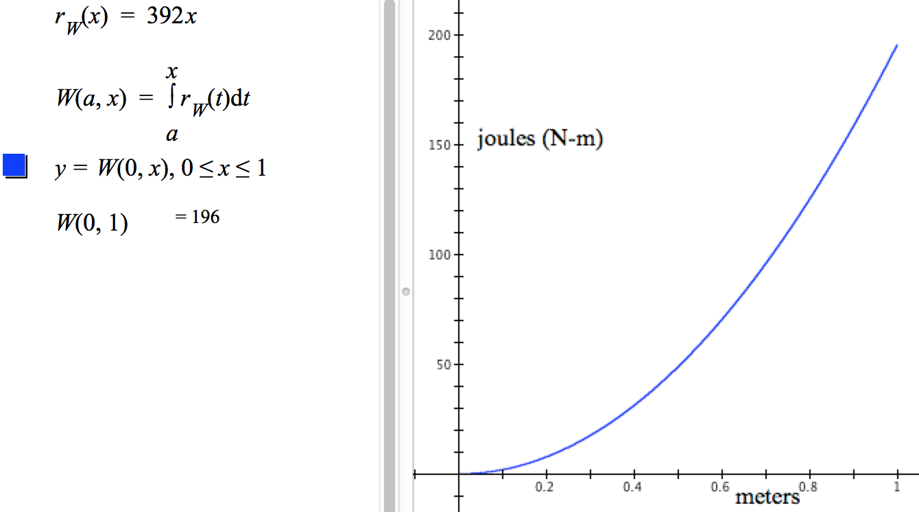
Figure 8.5.21. GC file to compute and graph work done to displace this spring x meters.
A right circular cylindrical barrel with radius $r=0.7$ m and height 1.3 m contains a fluid having density $\rho=750\text{ kg/m$^3$}$. Fluid is pumped from the barrel from the fluid's top surface and exits at the barrel's top edge. What work will be accomplished at every moment of emptying the barrel?
The scenario of emptying a fluid-filled barrel poses a complication that was not present in the platform scenario. We lifted the platform and cable all at once. We do not lift the fluid all at once. Instead, we can think of the fluid lifted in microscopic layers.
We need to understand that there are two things varying in this scenario:
Lifting the fluid in microscopic layers means that $dW$, the differential in work to empty the barrel, is the work done to lift one layer (see Figure 8.5.22).
Figure 8.5.22. The differential in work $dW$ is the work done to lift a microscopic layer of fluid to the barrel's top.
The differential in work $dW$ is made by a force acting through the distance from the fluid's surface to the barrel's top. The value of $h$ increases down, so $-h$ reflects both the distance and direction of the displacement.
The force itself is the weight of the layer that is lifted to the barrel's top, which is $dw=g\, dM$. Notice that $g$ is negative, which ends up making $dw$ negative, which makes $dW=-h\,dw$ positive.
Figure 8.5.22 unpacks the quantitative relationships that constitute $dW$, the differential in work to lift a thin layer of fluid to the barrel's top. It ends with $dW$ expressed as a multiple of $dh$, having the form $dW=m\, dh$ where $m=-hg\rho A(h)$.
This means that $-hg\rho A(h)$, the coefficient of $dh$, is the rate of change of $W$ with respect to $h$ at depth $h$.
Therefore, the accumulation function $W$ whose values give the work to empty the fluid from a depth of $a$ meters to a depth of y meters is$$\begin{align}r_W(h)&=-hg\rho A(h)\\[1ex]W(a,h)&=\int_a^h r_W(t)\,dt\end{align}$$
For the barrel in this example, $\rho=750 \text{ kg/m$^3$}$, $A(h)=\pi(0.7)^2\text{ m$^2$}$ for all values of $h$, and $g=-9.8$ (m/s)/s.
Figure 8.5.23 shows a GC file (click here) that implements this solution. It shows a graph of $y=W(0,x),\, 0\le x \le 1.3$ and it shows that the work to empty the barrel is approximately 9560.71 joules.
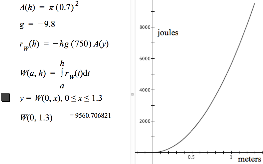
Figure 8.5.23. Accumulation of work to empty fluid from a barrel as the depth of the fluid's surface varies from 0 to 1.3 meters from the barrel's top.
Reflection 8.5.9. Use Figure 8.5.23 to answer this question:
Does half the work to empty the barrel empty half the barrel? Why "yes" or why "no"?
Pressure, like density, is a rate of change. Pressure is the rate of change of force with respect to the area to which it is applied. Pressure is measured in N/$\text{m$^2$}$ in the SI system and in $\text{lb/in$^2$}$ in the US system.
Figure 8.5.24 shows two footprints of the same truck tire. The left footprint encompasses an area of $13\cdot 5=85\text{ in$^2$}$ when the tire is inflated to 43$\text{ lb/in$^2$}$. This means that there is a force of $13\cdot 5\cdot 43=2795$ lbs being exerted on the ground by the truck through that tire.
The right footprint shows what happens to the tire when inflated to 100$\text{ lb/in$^2$}$. The footprint is smaller, but the force exerted on the ground is still 2795 lbs (You should check this for yourself.).
If all four tires are like this one, then each tire supports 2795 lbs and the truck weighs $4\cdot 2795=11,180$ lbs.

Figure 8.5.24. Two footprints of the same truck tire. (Left) The tire is inflated to 43$\text{ lb/in$^2$}$.
(Right) The tire is inflated to 100$\text{ lb/in$^2$}$.
Reflection 8.5.10. Why does it make sense that inflating a tire to a higher internal pressure makes the tire's footprint have a smaller area, yet $pressure\cdot area$ stays the same?
Figure 8.5.25 shows the world's largest aquarium window. The window's dimensions are:

Figure 8.5.25. World's largest aquarium window: 36.6 m wide and 8.3 meters high. The pool bottom extends 74.7 m from the window.
The water's weight exerts force on the window, and it exerts more force at deeper depths than at shallower depths.
What force does water exert on the portion of the window from the window's top to a depth $h$ meters from the top?
If a constant pressure $P$ is applied over an expanding area $A$, then $dF$, the differential in force as $dA$ varies is $dF=P\,dA$. This means, for example, that a pressure of 207 N/$\text{m$^2$}$ means that $dF=207\,dA$ N/$\text{m$^2$}$. As area varies by $dA\text{ m$^2$}$, the force applied to that area varies by $207\,dA$ Newtons.
It is often the case that we can model a situation so that area, a two dimensional quantity, varies by holding one dimension constant while the other varies. In a rectangle that has width $w$, height $h$, and area $A=w\cdot h$,$$\begin{align}dA&=w\,dh\qquad\text{if the rectangle's height is varying for a fixed width, or}\\[1ex]dA&=h\,dw\qquad\text{if the rectangle's width is varying for a fixed height}\end{align}$$
Water is incompressible, which means that the pressure at a depth of $h$ meters is the same in all directions and is the same regardless of the area to which it applies.
Enter $r_F$ and $F$ into GC, then enter $F(0,8.3)$. GC will report that the force on the entire window is $F(0,8.3)=12\,354\,732.6$ (Newtons), which is approximately 2,777,454.4 pounds. GC reports the force from 4.15 to 8.3 meters to be 9,266,049.45 Newtons.
Turn the beam around in Example 3, attaching the denser end to the fulcrum. Graph the torque exerted by the beam from the fulcrum to x cm from the fulcrum for all values of $x, 0\le x \le 250$. Why is the torque curve for the beam now different from the original one?
Define a function m such that $m(t)$ gives the culture's mass at each moment t of elapsed time, $t \ge 0$.
Compare the graph of $y=m(x)$ to the graph of $y=r_m(x)$. Explain how they are consistent with each other.
Why does the behavior of $y=m(x)$ make sense in terms of a bacterial culture in a growth medium?
Explain how you can think of any value of $15d(x), 0 \le x \le 24$ as the rate of change of the pool's volume with respect to distance from the pool's deep end.
What is the pool's total volume?
Approximately how far from the pool's deep end must you measure to get half the pool's volume?
Re-examine Example 5.
Explain why it makes sense, in terms of how the logistic rate of change function is defined, that a population with this rate of change at a moment has an inflection point at $t=0$. Interpret this inflection point in terms of population growth over time.
Verify graphically, using various values of L and k, that a population having a logistic rate of change always approaches a population of $L$ individuals. This is why L is called the carrying capacity of the population's environment.
Show that the point of inflection for a population having this logistic rate of change is always at $x=\dfrac{\ln C}{k}$.
A ball suspended by a 10-foot long rubber cord is at rest. It is given a sudden push downward; the cord stretches, then retracts, pulling the ball upward. (See the animation, below).
The ball's rate of change of displacement from rest is given by the function $r_d$, defined as $$r_d(t)=e^{-0.0625t}\left(0.25\sin(t)-4\cos(t)\right), 0≤t≤100$$where $r_d(t)$ is in ft/sec and t is the number of seconds since the ball was pushed.
Define a function $d$ whose graph $y=d(x)$ gives the ball's displacement from initial rest at each moment x seconds after being pushed.
Explain how your function gives the ball's net displacement at values of x.
Use your graph to determine the moments during the first 18 seconds that the ball's displacement reaches a local minimum. A local maximum.
Does the ball's displacement from rest have a global maximum? A global minimum?
Re-examine Example 6.
The National Football League has a policy that a stadium cannot serve beer past the end of the 3rd quarter. Each quarter of football lasts, on average, 0.75 hours, with a 0.25-hour break after the 2nd quarter.
Katie, who has a body mass of 50 kg, drank a 20-oz glass of beer during the first quarter of the game and another during the third quarter. She consumed each glass of beer in 4 equal amounts spread equally across a quarter of play, and she reached her car 30 minutes after the game ends. Can Katie legally drive home after the game? If not, how long must she wait?
The force of gravity on objects near Earth's surface is often approximated to be $F=m\cdot g$, where $m$ is the object's mass in kg and $g=-9.8$ (m/s)/s. However, for objects that are very large or very far apart you must calculate the force of gravity using $$F=\frac{-Gm_1m_2} {d^2}$$where $m_1$ is the first object's mass, $m_2$ is the second object's mass, $G=6.674⋅10^{-11}$ (N-m)/$\text{kg$^2$}$, and $d$ is the number of km between objects.
The earth's mass is $9.972\cdot 10^{24}$ kg. Imagine that we have a giant flagpole at the North Pole, 20,000 km high and cross sections of area 1 $\text{m$^2$}$. The flagpole's mass is $1.61⋅10^{11}$ kg and has uniform density.
How much does the flagpole weigh? That is, what is the accumulated gravitational force on the flagpole from the flagpole's base to a height of x km, $0\le x\le 20,000$? For convenience, assume that the Earth's mass is concentrated at its center, 6371 km from the pole's base.
The toy cars from Example 2 race again, but this time they have different accelerations: $$a_1(t)=\sin\left(\frac{3\pi t}{5}\right) \text{ (ft/sec)/sec, and }a_2(t)=\cos\left(\frac{2\pi t}{5}\right) \text{ (ft/sec)/sec.}$$
Write a GC file that you can use to compute work done in stretching any spring any displacement and to graph the spring's work function.
Write the GC file pretending that the only information you are given is one displacement (from any position) and the mass that caused that displacement.
Use your file to answer the question in the spring scenario.
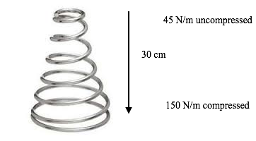
The conical spring shown below has variable stiffness. It's stiffness is 45 N/m when uncompressed, 150 N/m when fully compressed, and stiffness varies linearly with displacement from rest.
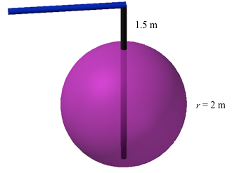
A spherical tank with radius $r=2$ m is full with a fluid that becomes denser from top to bottom. The fluid's density is $\rho(h)=600+(25h)^{1.3}\text{ kg/m$^3$}$, where $h$ is distance from top of the sphere.
The tank is emptied by pumping fluid to a height of 1.5 m above the tank's top.
Note: The radius $r_1(h)$ of a cross section at depth $h$ in the sphere's upper half is $r_1(h)=\sqrt{h(2r-h)}$, where $r$ is the sphere's radius. You will need to adjust this for the sphere's lower half.
| < Previous Section | Home | Next Section > |