Section 6.1
Approximate Rate of Change in Open Form
from Exact Accumulation in Closed Form

Review of Chapter 5

Chapter 5 addressed the problem of representing an accumulation function in open form when we have its rate of change function in closed form. Chapter 5 addressed the first foundational problem of calculus:

We will work backward from the end of Chapter 5 to develop techniques that start with an exact accumulation function in closed form and derive its exact rate of change function in closed form.

We will then close the loop regarding the relationship between exact accumulation functions in closed form and exact rate of change functions in closed form. We do this with the aim that we can recover one whenever we have sufficient information about the other.

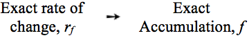
Figure 6.1.1 repeats the overview given in Chapter 5 of the journey from rate of change functions in closed form to accumulation functions in open form.

Figure 6.1.1 is a reminder of the method we developed in Chapter 5.

1. Start with an exact rate of change function $r_f$ in closed form. Its values gives the rate of change at every moment of an (unknown) exact accumulation function f.
2. Use the meaning of rate of change at a moment to assume that $r_f$ is essentially constant over small intervals of size $\Delta x$ that contained each moment.
3. The value of x varies through each $\Delta x$-sized interval. Each value of $dx$ produces a value $dy=m\,dx$, creating a piecwise-linear approximate net accumulation function A. Values $A(x)$ approximate $A_f(x)$, the exact net accumulation in f from a to x.
4. We said $A_f$ is the exact net accumulation function for $r_f$ when $\Delta x$ is so small that making it smaller has no appreciable effect on values of $A(x)$. We represented $A_f$ in open form as $A_f(x) = \int_a^x r(t)dt$.
5. Every value of $A_f(x)$ gives us the exact net variation in f from a to x, which is $f(x)-f(a)$. So $A_f(x)=f(x)-f(a)$, or $\int_a^x r_f(t)dt=f(x)-f(a)$. Another way to say the same thing is $f(x)=f(a)+\int_a^x r_f(t)dt$.

6.1.1 Exact Accumulation Functions in Closed Form

Chapter 6 will begin where Chapter 5 ended to address the second foundational problem of calculus:

Reflection 6.1.1. Compare the first and second foundational problems of calculus. How are they different? How are they related?

You have dealt with exact accumulation functions in closed form since at least 7th grade, without knowing it.

Any function g that gives an amount of quantity A in relation to an amount of quantity B is an exact accumulation function. We can think of any value $g(x)$ is the exact accumulation of the quantity it represents as the value of x varied up to its present value.

Example: Area of a square as an accumulation of variations in area

$f(x) = x^2, x \ge 0$ is an amount function. Every value of f gives an amount of area enclosed within a square with side-length x.

When the square’s side length is 13.327 inches, its area is $f(13.327)=13.327^2$ , or 177.609 $\mathrm{in}^2$. The area of a square with side length x inches is $f(x)=x^2$ square inches. .

We can think of f as an accumulation function.

For any given side length x, we can think of the square’s side as having grown in length from $t=0$ to $t=x$.

Thinking of the side length varying means that the square itself varies. The square’s area will grow as t varies from 0 to x inches.

Figure 6.1.2 shows f(15) in terms of the area of the square accumulating as its side length varies from 0 to 15.

The first pass in Figure 6.1.2 shows area accumulating as differentials in the side length vary within intervals of size 1 inch. The second pass shows area accumulating as differentials in side length vary within intervals of size 0.2 inch.

Do not think of area of the square in this example just as a function of the square's side length. Rather, think of area as an accumulation of variations in area that are made at some rate with respect to variations in the square's side length as the side length varies from $t=0$ to $t=x$.

In other words, think of $x^2$ as

where $r_f(t)$ is a function that gives the exact, momentary rate of change of the square’s area with respect to its side length for every value of its side length. Notice: At this moment we do not know the definition of $r_f$ so that $x^2 = \int_a^x r_f(t)dt$. But, we can presume there is such a function $r_f$ and try to devise a method to determine it.

"Open Form" versus "Closed Form" definitions

In the example above, we ended by stating $x^2=\int_a^x r_f(t)dt$ for some rate of change function $r_f$. The left side ($x^2$) is said to be in closed form. The expression tells you how to compute a value. The right side $\left( \int_a^x r_f(t)dt \right)$ is said to be in open form. You know what the expression means, but the expression doesn't tell you how to compute a value. However, both expressions define the same accumulation function.

In principle, we will speak of a function being defined in "open form" when the definition itself emphasizes the function's meaning. We will speak of a function being defined in "closed form" when the definition emphasizes how to compute values of the function. A common goal in mathematics is to define a function both ways—in terms of its meaning and in terms of computing its values.

In Chapter 5, we started with exact rate of change functions defined in closed form and ended with exact accumulation functions defined in open form. We relied on GC to compute values of the open form integrals we ended with.

The aim of this chapter is to develop methods that will allow us to start with any exact accumulation function defined in closed form and determine the exact rate of change function from which it came, also defined in closed form.

Then you will also learn that an accumulation function’s rate of change function gives you many insights into a situation that the accumulation function models.

Not every function can be thought of as being built from a rate of change function. The Blancmange and Weierstrass functions from Section 4.8 had no moments at which they varied at a rate that was essentially constant. It is therefore not possible to think of any value of either the Blancmange or Weirstrass function as having accumulated.

We will address this matter in more detail later. For the meantime, we will concentrate on functions that can be viewed as accumulation functions that come from some quantity accumulating at some rate of change at almost every moment of their independent variables.

Reflection 6.1.2. Remind yourself of what the word "exact" means when we speak of an exact rate of change function and an exact accumulation function.

Reflection 6.1.3: Remind yourself of what the terms "open form" and "closed form" mean when we speak of a function defined in open form or a function defined in closed form.

6.1.2 Reversing the Process: Deriving Exact Rate of Change from Exact Accumulation

Overview of Accumulation from Rate

The focus of Chapter 5 was to develop and understand the mathematics of determining an exact accumulation function from an exact rate of change function given in closed form. This endeavor addressed the first foundational problem of calculus:

Our efforts in Chapter 5 involved this process:

This process ended with the integral, an open form representation of the net variation in the exact accumulation function f from a to x that is built from $r_f$:$$A_f(x)=\int_a^x r_f(t)dt$$

The integral function was the culmination of the 4-step process. It achieved the desired result in one step:

Reversing the Process

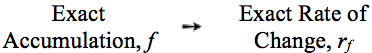
To derive an exact rate of change function in closed form from an exact accumulation function in closed form, we must reverse the process that we developed in Chapter 5. In doing so, we will address the second foundational problem of calculus:

You know how much of a quantity there is at every moment; you want to know how fast it is varying at every moment.

The method for reversing the process developed in Chapter 5, of going from an exact rate of change function to an exact accumulation function, entails these steps:

Our final goal is to develop a method that accomplishes the three steps listed above in one step. That is, we aim to derive the exact rate function directly from a given exact accumulation function:

Here is an outline of our quest:

• We are given a function f in closed form.
• Interpret f as being an accumulation function. Each value $f(x)$ represents an amount that has accumulated in $f$ up to the value of x. The net variation in in $f$ from $t=a$ to $t=x$ as $f$ varied at a rate $r_f(t)$ at each moment t is therefore,$$\color{red}{\text{(Eq. 6.1.1)}}\qquad \text{net variation in $f$ from $a$ to $x$ }=\int_a^x r_f(t)dt$$
• Our goal is to recover $r_f$ in closed form.

Reversing the accumulation process requires that we have the accumulation process itself firmly in mind. You would be wise to revisit the introduction and its description of Figure 6.1.1 before continuing.

Figure 6.1.3 gives a visual summary of the approach we will develop to approximate an accumulation function’s rate of change function, which we explain after the animation.

The highlighted points on the graph of f in Figure 6.1.3 are the values of f at the left end of each $\Delta x$-interval.

Each interval has a width of $\Delta x$. The piecewise linear function (call it g) over each $\Delta x$-interval in the left graph of Figure 6.1.3 produces the same variation over that interval as does f. Its constant rate of change over any $\Delta x$-interval containing a moment of x will be the value of $r(x)$ once we define r appropriately.

Therefore, the conceptual definition of g is

$$\color{red}{\text{(Eq. 6.1.2)}}\qquad g(x) = r(x)\left(x-\mathrm{left}(x)) + f(\mathrm{left}(x)\right)$$

The graph of g over any $\Delta x$-interval passes through the points $(\mathrm{left}(x), f(\mathrm{left}(x))$ and $(\mathrm{left}(x+\Delta x), f(\mathrm{left}(x+\Delta x))$, and has a constant rate of change over that interval.

Therefore, the approximate rate of change of g over any $\Delta x$-interval containing a moment of x will be the average rate of change of f over the interval containing this value of $x$.

The average rate of change of f over the $\Delta x$-interval containing this value of $x$ is the variation in f over that $\Delta x$-interval divided by the value of $\Delta x$, the variation in x over that interval.

This average rate of change is the value of $r(x)$, the rate of change of g (the piecewise-linear approximation of f) over the interval containing this value of $x$.

In symbols, $r(x)$, the constant rate of change of the function g over any $\Delta x$-interval containing the moment $x$, is $$\color{red}{\text{(Eq. 6.1.3)}}\qquad \begin{align}r(x) &= \frac{f\left(\mathrm{left}(x))+\Delta x\right) - f\left(\mathrm{left}(x)\right)}{(\mathrm{left}(x)+\Delta x)-\mathrm{left}(x)}\\[1ex]&= \frac {f(\mathrm{left}(x)+\Delta x) - f(\mathrm{left}(x))}{\Delta x}\end{align}$$

6.1.3 Your Turn

Part 1 — By hand

Use a printout of this graph with the following activity. Note: An interval $a≤x≤ b$ is also represented as $[a,b]$.

• The printout contains a graph of $y=f(x)$ with $\Delta x=0.9$. The ordered pairs $(-1, 1.7)$, $(-0.1, 2.7)$ and $(0.8, 2)$ are on the graph.
• Highlight the two $\Delta x$-intervals of length 0.9 that comprise the interval $ [‑1, 0.8]$.
• How much does f vary over the first interval? The second interval? Represent each variation symbolically and numerically.
• Does f vary at a constant rate of change or at a varying rate over each interval? How can you tell?
• What is the constant rate of change over the first $\Delta x$-interval that another function g would need to produce the same variation as produced by f? Represent this constant rate of change symbolically and numerically.
• What is the constant rate of change over the second $\Delta x$-interval that another function g would need to produce the same variation as produced by f? Represent this constant rate of change symbolically and numerically.
• Define the function r so $r(x)$ is the rate of change of g at each moment of x in $[-1, 0.8]$. Sketch a graph of r over the interval $[-1, 0.8]$.
• Define the function g so $y=g(x)$ coincides with the piecewise approximation to the function f over the interval $[-1,0.8]$.
• What is the numerical value of $r(0.25)$? What does the value $r(0.25)$ represent? Is it the same as $f(0.25)$? Explain.

Part 2 — Using GC.

Save your GC file with this work. You will use it in Exercise Set 6.1.3.
Mac users: Type "\option-j x\" to get "$\Delta x$". Windows users: Type "\Dx\" whenever you see "$\Delta x$".

1. Define f as $f(x)=e^{\cos x}$.
2. Enter $a = -1$, $\Delta x = 0.2$ on one line (type the comma, too).
3. Define the function left as left$(x) = a + \Delta x \left\lfloor \dfrac{x-a}{\Delta x} \right\rfloor$. Reminder: Type "\left\" when defining left(x). Type "floor (x-a)/$\Delta x$" to get $\left\lfloor \dfrac{x-a}{\Delta x} \right\rfloor$.
   Remind yourself of what a value of left(x) means for given values of a and $\Delta x$.
4. Define g and as in Equation 6.1.2. Define r as in Equation 6.1.3.
5. Enter $y=f(x), a \le x$ on one line.
6. Enter $y=g(x), a \le x \le n$ on a second line.
7. Enter $y'=r(x'), a \le x' \le n$ on a third line. The prime (') notation tells GC to display the graph in a second graphing pane.
8. Click "n" on the n slider. Set lower and upper values to -1 and 8, respectively.
9. Click the play button on the n slider. You should see a replay of Figure 6.1.3, except that you might see calculator drool in your graph of $y'=r(x')$.
10. Explain in terms of the functions f, g, and r, and their displayed graphs, what is happening on your screen.

Exercise Set 6.1.3

1. For each function in a-e,
   • Let $\Delta x=0.25$ and a=1
   • Define the function’s approximate rate of change function r in GC as in Equation 6.1.3.
   • Evaluate r for three values of x in the intervals (2.25, 2.5] and (3.75, 4.0]. What do you notice? Why?

2. What did each value of r that you found in Exercise 1 mean? Do this for each particular value you found until you can give a general meaning that covers them all.

Use your file from Part 2 above to answer exercises 3-6, but hide the graphs. The following exercises assume you defined f, g, and r successfully.

3. In GC, enter $g(0.5)$. You should get 2.3973 (to 4 decimal places). What does this number mean?
4. In GC, enter $r(0.5)$. You should get -1.14654 (to 4 decimal places). What does this number mean?
5. In GC, enter $y=g(x), a ≤ x ≤ a + \Delta x$. Interpret this graph.
6. In GC, enter $y'=r(x'), a ≤ x' ≤ a + \Delta x$. Interpret this graph.
7. Select New in the File menu to open a new GC file. In each of a. - d., you are given a function f. Define g and r  as in Equations 6.1.2 and 6.1.3. Enter $g(c)$ and $r(c)$ on separate lines for three different values of c. Interpret the values that GC displays each time.
1. $f(x) = \sin(x)$


2. $f(x) = \sin(x) e^{\cos x}$


3. $f(x) = x(x-1)(x+1)$


4. $f(x) = x \sqrt{\sin x}$. For what values of x are g and r defined?


8. The left side of the figure below shows graphs of $y=f(x)$ in aqua, $y=g(x)$ in magenta. The right side shows the graph of $y=r(x)$ in red, with a point on the graph of $y=r(x)$ highlighted. What do the coordinates of the highlighted point represent about the graph of $y=g(x)$?




9. Give a detailed explanation of what the animation in Figure 6.1.3 shows.

6.1.4 Smoothing the Approximate Rate of Change Function

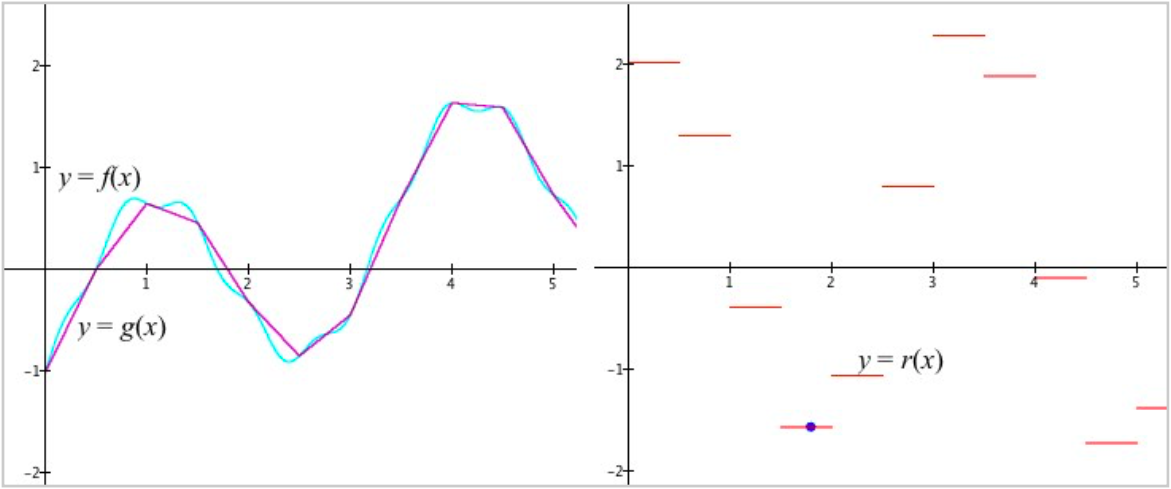
The method outlined in Section 6.1.2 above, Reversing the Process, indeed produces an approximate rate of change function r for an exact accumulation function f. However, if f is not linear, then r is discontinuous from one $\Delta x$-interval to the next.

Consider the diagram below and think about why r is discontinuous from one $\Delta x$-interval to the next. What would the displayed graph of r look like over the interval [-1,0.8)?

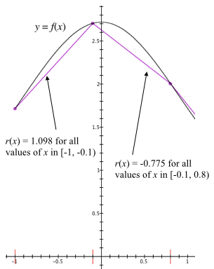
The reason for the discontinuities in $r(x)$ is because when f is not linear, values of $r(x)$ will "jump" from a constant value within one $\Delta x$-interval to a different value at the beginning of the next $\Delta x$-interval.

We can solve the problem of discontinuities in the values of r with a simple change of technique.

Instead of chopping the domain of x into successive intervals of length $\Delta x$, we can use a technique introduced by David Tall. It is to slide one interval of length $\Delta x$ along the axis.

The value of r for any value of x will be the constant rate of change over the interval $[x, x+\Delta x]$ as the value of x varies.

Figure 6.1.4 illustrates this change of technique. It starts with the technique of using fixed intervals of length $\Delta x$. It then displays the "sliding interval" technique, using intervals of length 1, 0.1, and 0.01.

Reflection 6.1.4.1: Why does the graph of the approximate rate of change function defined with a sliding interval always go through the left endpoints of the parts of the fixed-interval rate of change function’s graph? Does this happen also in the animation when $\Delta x$ = 0.01?

Reflection 6.1.4.2: Consider again why in Figure 6.1.4 the graph of the fixed-interval rate of change function (in blue) is discontinuous, while the graph of the sliding interval rate of change function (in red) is continuous.

The sliding interval technique has a huge benefit. Not only does the sliding interval produce a continuous function, the definition of r is simpler. Before introducing sliding intervals, the definition of r as the approximate rate of change function for f is repeated below as Eq. 6.1.5:$$\color{red}{\text{(Eq. 6.1.5)}}\qquad \begin{align}r(x) &= \frac{f(\mathrm{left}(x))+\Delta x) - f(\mathrm{left}(x))}{(\mathrm{left}(x)+\Delta x)-\mathrm{left}(x)}\\[3ex]&= \frac {f(\mathrm{left}(x)+\Delta x) - f(\mathrm{left}(x))}{\Delta x}\end{align}$$

With the sliding secant, the definition of r is of the constant rate of change over the interval that starts at the current value of x, not left(x), and which has a length of $\Delta x$. The simplified definition of r is

$$\color{red}{\text{(Eq. 6.1.6)}}\qquad \begin{align}r_2(x) &=\frac {f(x+\Delta x) - f(x)}{(x + \Delta x) - \Delta x}\text{, or simpified,}\\[2ex] r_2(x) &=\frac {f(x+\Delta x) - f(x)}{\Delta x}\end{align}$$

As a look ahead, Figure 6.1.5 compares the graphs of $r_2$ and the exact rate of change function $r_f$ as $\Delta x$ gets very small.

Visually, the graph of r in the right pane appears to move atop the graph of $r_f$. This suggests that $r_2$ produces good approximates of $r_f$ for sufficiently small values of $\Delta x$.

The right side of the animation in Figure 6.1.5 might suggest to you that the graph of $r_2$ moves sideways as $\Delta x \to 0$. Examine the definition of $r_2$ in Equation 6.6. For each value of x, $f(x+\Delta x)$ approaches the value of $f(x)$ as $\Delta x$ gets smaller. Therefore, the values of $r_2$ must be moving vertically (up or down) as values of $\Delta x$ become smaller.

Figure 6.1.6 confirms that points on the graph of $y =r_2(x)$ move vertically as $\Delta x \to 0$. The graph of $r_2$ does not move sideways. Rather, it changes shape because the graph's points move up or down as the value of $\Delta x$ changes.

We will use the definition of $r_2$ as our standard definition of r, the approximate rate of change function for a given accumulation function. To repeat, from here forward, $$r(x)=\frac{f(x+h)-f(x)}{h}$$ will be our standard definition of a function f’s approximate rate of change function.

Alert: From now on, we will use "h" in place of "$\Delta x$" so that Mac and Windows users can type the same thing.

Exercise Set 6.1.4

1. Go through the following steps for both (a) and (b).
   
1. Examine the displayed graph of f.
2. Imagine what the graph of $r_f$ might look like based on the behavior of f’s graph.
3. iii. Make a hand-drawn sketch of the graph you anticipate for $r_f$.
4. iv. Enter the definition of f and r into GC and compare GC’s graph of r with your hand-drawn sketch.
5. v. Click on a point of r’s displayed graph. Write the point’s coordinates and an explanation of what they mean.
2. The total cost C of producing p units of a widget depends upon p.  Economists use the term marginal cost for the rate of change of the total cost with respect to the number of units produced.  The function C, defined as $C(p)=200+5 \sqrt{30p}$, models the cost of producing p items at a particular factory.
1. n GC, graph $y=C(x)$ (scale the axes appropriately). What do you notice about the cost of goods as p increases?
2. Define $r(p)$, the approximate rate of change function for C (consider what would be a logical value for h).
3. Enter $y’=r(x’)$ so that GC displays the graph of r in its right pane. What is the approximate marginal cost when $p=15$?
4. How does the marginal cost vary as the number of units produced varies? Why does this make sense? (Adapted from Kline p. 35)
3. A species of bacteria is being researched in laboratory settings.  Researchers are testing a new disinfectant. They start a bacterial culture with a mass of 5 grams and allow the culture to grow for several hours. Then they release the disinfectant after 20 hours. The bacteria will begin to die off once the disinfectants are released. The function b, defined below, models the number of grams of bacteria in the petri dish t hours after the culture is started.

$$b(t)=5(1.25^{t/3}-d(t)) \text { if } t \ge 0,\\[1ex] d(t)=\left\lbrace \begin{align} &1.4^{(t-20)/2}-1 \text{ if } t \ge 20 \\ &0 \text{ if } t \lt 20 \\ \end{align} \right.$$

1. Trace the graph of $y=b(x)$ in GC to determine the culture's maximum mass.  After how many hours  does the culture reach this maximum?
2. According to this model, when will the bacteria have vanished?
3. In GC, graph y = r(x), the approximate rate of change function for b. What is true about the value of r(x) at the moment that the bacterial culture reaches its maximum mass? Why is it reasonable that r(x) would have that value?
4. Save your GC file for this exercise. You will need it in the next exercise.
   
   For each of a) through c), use GC to graph each function’s approximate rate of change function.  Let $h=0.01$.  Each of these graphs will approximate the graph of a function that should be familiar to you. What is the familiar function in each case?
   1. $f(x) = \mathrm{ln}(x)$
   2. $f(x) = \cos(x)$
   3. $f(x) = e^x$
5. Click on a point on each of the approximate rate graphs you made in 4.a, 4.b, and 4.c. Record its coordinates. State what the point’s y-coordinate means in relation to the value of its x-coordinate.

6.1.5 Relating Rate of Change and Accumulation

In section 6.1.4 we determined that the function $r(x)=\frac{f(x+h)-f(x)}{h}$ approximates an exact accumulation function f’s exact rate of change function. Each value $r(x)$ is an approximation to f’s rate of change at a moment x.

If this is indeed true, then the function F defined as $F(x)=\int_a^x r(t)dt$ for some number $a$ should approximate the net variation in the function f  from a to x. We will check to see that this is true and explore why it is true.

First let’s consider the meaning of a in $\int_a^x r_f(t)dt$. It is the initial value of x from which a variation in exact accumulation is measured.

Since f is an exact accumulation function built from its rate of change function $r_f$, the accumulation $\int_a^x r_f(t)dt$ is starting at $f(a)$. Likewise, we know from Chapter 5 that $\int_a^x r_f(t)dt = f(x)-f(a)$ and therefore $f(x)=f(a)+\int_a^x r(t)dt$. These observations will be important right away.

Let the function f be defined as $f(x)=x^2+1$. We can think of it as an exact accumulation function, such as the area of two squares, one of side length 1 and the other of side length x. f's approximate rate of change function r is defined in open form as $$r(x)=\frac{f(x+h)-f(x)}{(x+h)-x},$$ or more simply as $$r(x)=\frac{f(x+h)-f(x)}{h}.$$The smaller the value of h, the better the approximation that r is to $r_f$.

Figure 6.1.7 examines the graph of the function F defined as $F(x)=\int_a^x r(t)dt$ and compares it to the graph of the function f.

The animation in Figure 6.1.7 suggests that r defined as $r(x)=\frac{f(x+h)-f(x)}{h}$, for small values of h, approximate f’s exact rate of change function $r_f$.

At the beginning of Figure 6.1.7 we graphed $y = F(x)$, where $F(x)=\int_a^x r(t)dt$ and $a = -2$. The graph appeared to be congruent to the graph of $y = f(x)$ but differed by a constant (it was shifted vertically).

When we graphed $y = f(a) + F(x)$, the two graphs coincided. This says that f, the exact accumulation function we started with, can be recovered by integrating r. This means that r indeed is an approximation to $r_f$, f’s exact rate of change function.

The function r is defined in open form. At this moment, we do not have a closed form representation of $r_f$. In Section 6.2 we will learn to derive closed form representations of exact rate of change functions when given their exact accumulation functions in closed form.

Exercise Set 6.1.5

Exercises 1-6 refer to the GC file displayed in Figure 6.1.7.

1. In GC, enter the statements listed in Figure 6.1.7. Now do this:
2. Make a list on a sheet of paperof 5 other definitions for f, each of your choosing. 
3. Change the definition of f in Figure 6.1.7 to each definition you listed, one by one.
   
4. Answer this question: Why does the definition of f not matter in terms of whether the graph of $y=f(x)$ coincides with the graph of $y=f(a)+\int_a^x r(t)dt$
5. Change the second line to h = slider(0.001,1). Change the value of h. How does the value of h affect the graph of F?
6. Enter $y'=r(x')$. This makes GC display a graph of r in the right graphing pane. Click on a point on the graph of r. Write the coordinates of that point and explain what those coordinates mean.

Questions 7 - 11 are based on the animation in Figure 6.1.7.

7. At the beginning of the animation, the vertex of the graph of $y=F(x)$ moved up to touch the x-axis as the value of a increased to 0, then the graph moved down as the value of a increased beyond 0. Why did the graph's vertex not rise above the x-axis as the value of a increased?
8. The value of a is -2 at the beginning of the animation. When $a=-2$ the graphs of $y=F(x)$ and $y=f(x)$ differ by a constant, meaning that there is some number C so that $f(x)-F(x)=C$. What is C?
9. Why did the graph of $y = F(x)$ move as it did when the value of the a slider varied. Does the value of a effect r’s approximation of $r_f$?
10. $F(x)=\int_a^x r_f(t)dt$. The graph of $y=f(a)+F(x)$ coincided with the graph of $y=f(x)$ regardless of the value of a. Why? What does this imply about $\int_a^x r_f(t)dt$?