Section 7.2
Higher Order Rate of Change Functions

Suppose h is a function with a rate of change function $r_h$. The function $r_h$ is a function, so we can inquire about its rate of change function, $r_{(r_h)}$.

Suppose $r_h$ has a rate of change $r_{r_h}(k)$ at the moment $x=k$. Then $r_{(r_h)}(k)$ can give us, in principle, the same kind of information about the behavior of $r_h(x)$ around $x=k$ as $r_h(k)$ gives us about the behavior $h(x)$ around $x=k$.

When $r_{(r_h)}(x)$ is positive at $x=k$, $r_h$ is increasing over an interval containing the value of k; when $r_{(r_h)}(x)$ is negative at $x=k$, $r_h$ is decreasing over an interval containing the value of k. When $r_{(r_h)}(x)=0$, or $r_{(r_h)}(x)$ is undefined at $x=k$, then $r_h$ has all the possibilities we investigated for $r_h$ in relation to h.

Notation

In line with the different notations for rate of change functions introduced in Chapter 6,we can represent higher order rate of change functions in three ways. Each notation has strengths and weaknesses.

Let k be a function defined as $k(x)=2\sin(x)e^x$. Then we can represent $r_f$ and its rate of change function in three ways:

Reflection 7.2.1. Confirm for yourself that $\dfrac{d}{dx}\left(2\sin(x)e^x\right)=2e^x\left(\sin(x)+\cos(x)\right)$ and $\dfrac{d^2}{dx^2}\left(2\sin(x)e^x\right)=4e^x\cos(x)$

Exercise Set 7.2.1

1. Find the $n^{th}$-order rate of change function for each of the following functions. Represent each using rate notation, differential notation, and prime notation.

Function	$n$	$n^{th}$-order rate of change function
$f(x)=x^5-x^2-\cos(x)$	2
$g(t)=\sin(t)e^{2t}$	3
$j(p)=\ln(p)$	2
$k(y)=y^{10}$	6

Applications of Higher Order Rate Functions

Second- and third-order rate of change functions have direct applications in the sciences, in economics, and in characterizing behaviors of functions in general. In Chapter 10, we will use higher order rate of change functions to develop methods to approximate values of functions we cannot compute directly.

Acceleration

Acceleration, as a quantity, is often associated most closely with mechanics. If an object is "speeding up", a natural question is, "At what rate is it speeding up?". For example, suppose an object at rest "speeds up" at a constant rate to a velocity of 15 m/sec over a period of 5 seconds. At what rate did it speed up? It increased its velocity at the rate of 3 m/sec every second, or 3 (m/sec)/sec.

Acceleration at a moment is the rate at which a rate of change function varies at that moment.

Mechanical force is defined in terms of an accelerated mass, or $F=ma$, where m is a measure of mass, typically in kg, and a is the object's acceleration, typically in (m/sec)/sec. A Newton is the force required to accelerate a mass of 1 kg at a rate of 1 (m/sec)/sec.

We could represent forces using the language of rate of change functions. If $s(t)$ represents a number of meters traveled in t seconds, then instead of $F=ma$ we could write

• $F(t)=m\dfrac{d^2}{dt^2}s(t)$,
• $F(t)=m\cdot r_{(r_s)}(t)$,
• $F(t)=m\cdot r_s^{(2)}(t)$,
• $F(t)=m \cdot s''(t)$.

They all say the same thing -- force is the product of a mass and the rate at which its velocity varies.

We also often speak of economic quantities in terms of acceleration: "How fast is inflation varying at this moment?" Inflation is a rate of change of the cost of goods. To ask how fast it is varying is to ask about how the price of goods is accelerating.

Notice that the concept of accleration can be applied broadly. We could speak of the rate at which an object's acceleration accelerates.

Jerk

Imagine you are a water skier, waiting in the water for the boat to pull the rope taught and accelerate to top speed (see Figure 7.2.1). Your arms will hurt if the boat accelerates too rapidly. That "hurt" is due to the boat trying to accelerate your body to top speed in a short period of time.

The rate at which you accelerate is called jerk. Let $s(t)$ represent how far the boat pulls you from a stationary position in t seconds. The jerk you experience t seconds after the rope becomes taught is represented in differential notation by $\dfrac{d}{dt}\left(\dfrac{d^2}{dt^2}s(t)\right)=\dfrac{d^3}{dt^3}s(t)$, or in rate notation by $r_{\left( r_s^{(2)}\right)}(t)=r_s^{(3)}(t)$.

Figure 7.2.1. (Left) Water skier waiting for the boat to accelerate him to top speed. (Right) Skiing at top speed.

Drag racing drivers experience jerk similarly to water skiers. The dragster in Figure 7.2.2 accelerated from 0 mi/hr to 329.21 mi/hr in 3.728 seconds, for an average acceleration of 88.31 (mi/hr)/sec. If its acceleration was constant, the jerk would be 0 (no change in acceleration during the race).

However, acceleration at the beginning of the race is far greater than at the end. A dragster can reach 100 mi/hr (161 km/hr) from start in 0.8 sec, but can take 2.2 sec from start to reach 200 mi/hr (322 km/hr).

The dragster's average acceleration in the first 0.8 sec is $\dfrac{100}{0.8}\text{ (mi/hr)/sec }$in its first 0.8 seconds while its average acceleration is $\dfrac{100}{1.4}\text{ (mi/hr)/sec }$in its next 1.4 seconds.

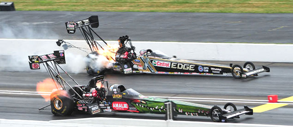
Figure 7.2.2. A dragster at the end of its race. The record for 1/4 mile (0.40 km) is 3.58 seconds with a top speed of 386 mi/hr (621.2 km/hr).

Behavior of Functions

Suppose f is a function of x and it has a rate of change at every moment in an interval I. In Section 7.1 you learned you can tell whether the function is increasing or decreasing at the moment $x=k$ in I by examining the sign of its rate of change function $r_f(x)$ at $x=k$:

• If $r_f(x)$ is positive at the moment $x=k$, then f is increasing around $x=k$.
• If $r_f(x)$ is negative at the moment $x=k$, then f is decreasing around $x=k$. 
• If $r_f(x)$ is 0 at $x=k$, then we need to examine whether the sign of $r_f(x)$ changes as x varies near $x=k$.

Unfortunately, when $r_f(x)$ is not zero, we have no information about the way f is increasing or decreasing. Figure 7.2.3 illustrates this ambiguity. Both functions f and g are increasing over the interval $x>0$. However, while f increases, the value of $r_f$ also increases, whereas as g increases, the value of $r_g$ decreases.

Figure 7.2.3. Both f and g increase in value as the value of x increases over the interval $x>0$. However, as the value of x increases, the value of $r_f(x)$ increases but the value of $r_g(x)$ decreases.

Remember $r_f$ and $r_g$ in Figure 7.2.3 are also functions of x, so we can look at the sign of their (i.e., $r_f$'s and $r_g$'s) rate of change at a moment to see whether they are increasing or decreasing at that moment.

Let's examine the first- and second-order rate of change functions for f as defined in Figure 7.2.3.

\begin{align}\frac{d}{dx}\left(x^2+1\text{ if }x>0\right) &= 2x\text{ if }x>0\\[2ex]
\frac{d^2}{dx^2}\left(x^2+1\text{ if }x>0\right) &= \frac{d}{dx}2x\text{ if }x>0\\[2ex]
&= 2\text{ if }x>0 \end{align}

Since $r_{(r_f)}(x)$ is positive for all values of $x>0$, $r_f$ is increasing for all values of $x>0$. The function f is therefore increasing over the interval $x>0$, and its rate of change is increasing over $x>0$

Now let's do the same for g as defined in Figure 7.2.3. \begin{align}\frac{d}{dx}\left(\sqrt{x}-3\text{ if }x>0\right) &= \frac{1}{2}x^{-1/2}\text{ if }x>0\\[2ex]
\frac{d^2}{dx^2}\left(\sqrt{x}-3\text{ if }x>0\right) &= \frac{d}{dx}\left(\frac{1}{2}x^{-1/2}\right)\text{ if }x>0\\[2ex]
&= -\frac{1}{4}x^{-3/2}\text{ if }x>0\\ \end{align}

Since $x>0$, $-\dfrac{1}{4}x^{-3/2}$ is negative for all values of x, and therefore $r_g(x)$ is decreasing for all values of $x>0$. The function g is therefore increasing over the interval $x>0$, but its rate of change is decreasing over $x>0$.

There are standard terms for describing functions' behavior that are based on a function's second-order rate of change (the rate of change of its rate of change function).

Two cases many people find confusing

Play the animation in Figure 7.2.4.

How would you describe the behavior of the red graph that is tangent to the graph of $y=f(x)$ at $x=k$ as k varies (Figure 7.2.4, Left)?

Many people describe the red graph as having a rate of change that gets smaller (less steep), equals zero, and then gets larger. However, if you look at the value of $r_f(k)$ as k varies, you will see it is always getting larger. This is because a sequence of numbers like -10, -9, -8, ..., -1, 0, 1, 2, 3, ... is increasing. Each term is larger than the one preceding it.

Reflection 7.2.3. Describe the behavior of the graph in the right side of Figure 7.2.4. How does its rate of change vary as the value of k varies.

Reflection 7.2.4. Determine $\dfrac{d^2}{dx^2}$ of both f and g as given in Figure 7.2.4. What do their values tell you about $r_f$ and $r_g$? About f and g?

Points of Inflection

Suppose f is a function, and $r^{(2)}_f(k)$=0. If $r^{(2)}_f(x)$ is continuous and changes sign around $x=k$, then f is said to have a point of inflection at $x=k$.

Another way to put this is f has a point of inflection at $x=k$ if $r_f(x)$, the rate of change of $f$ with respect to x, changes from increasing to decreasing or from decreasing to increasing around $x=k$.

A consequence of $r_f(x)$ changing from increasing to decreasing or decreasing to increasing is $f''(k)=0$ and $f''(x)$ changes sign around $x=k$.

The function q defined as $q(x)=(x-2)^3+2$ has a point of inflection at $x=2$: $$\begin{align}q'(x)&=3(x-2)^2\text{, so }q'(2)=0\\[1ex]q''(x)&=6(x-2)\text{, so }q''(2)=0\\[1ex]\text{Finally, } q''(x)&\text{ changes sign from negative to positive around $x=2$}\end{align}$$Therefore $q'(x)$ changes from decreasing to increasing, making a point of inflection at $x=2$. The graph in Figure 7.2.5 illustrates this.

Figure 7.2.5. Function f has a point of inflection at x=2.
$f'(2)=0$, $f''(2)=0$, and $f''(x)$ changes from negative to positive around $x=2$.

Reflection 7.2.6. Explain the significance of $r_{(r_f)}(x)$ varying from negative to positive as x increases around $x=2$ in Figure 7.2.5.

Summary

Higher order rate of change functions are used in defining physical quantities like force, acceleration, and jerk. They are also useful for characterizing the behavior of functions by characterizing the behavior of their rates of change functions. In the case of behaviors of functions in general.

The table given below summaries the information you can glean by looking at values of first- and second-order rate of change functions in combination.

Exercise Set 7.2.2

1. We noted above that one can speak of the rate at which an object's acceleration accelerates. Suppose f is an accumulation function. Represent the rate at which the acceleration of f accelerates as $r_f^{(n)}(x)$. What is the value of n?
2. Determine the first- and second-order rate of change functions for each of the following. Check your work by using GC to graph the function's approximate rate of change function.
   
   Represent each first- and second-order rate of change function using rate notation, differential notation, and prime notation. State any necessary restrictions on a function's independent variable.

1. $f(x)=(\ln x)\cos(x^2)$

2. $g(x)=e^{\sin(x)}$

3. $h(x)=g(f(x))$, where g and f are defined as above.

4. $k(x)=\log(\cos(x))$

3. Sketch graphs that illustrate each of the ambiguities noted in the third column of Table 7.2.1

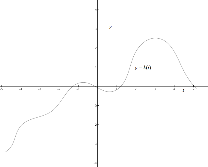
4. The graph of $y=k(t)$ for a function k is displayed below. Over what intervals, approximately, is $k'$ increasing? Decreasing?
   

5. Harry gave his sister the three displayed graphs shown below--one of $y=f(x)$, one of $y=f'(x)$, and one of $y=f''(x)$. But Harry did not say which graph was which. Which is which? Explain your answer.
   
   
   
   $y=f(x)$ is ______                $y=f'(x)$ is ______               $y=f''(x)$ is ______

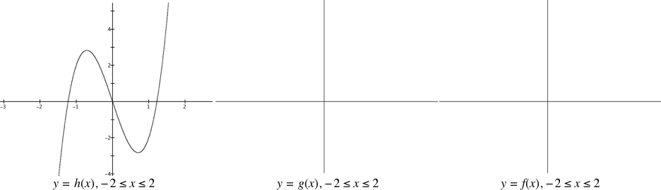
6. The graph of a function h is displayed below. Complete the tables below, giving approximate values where $h'$ and $h''$ are zero, and giving approximate intervals over which $h'$ and $h''$ are increasing or decreasing.
   

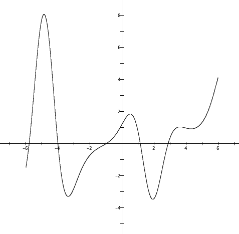
   h' is zero at these values of its independent variable	h' is increasing over these intervals	h' is decreasing over these intervals

   h'' is zero at these values of its independent variable	h'' is increasing over these intervals	h'' is decreasing over these intervals

   
   
7. There are two parts to this question.
   
   
1. Three functions, f, g, and h are defined over the interval $[-2,2]$; where $g(x)=f'(x)$ and $h(x)=g'(x)$. Also, $g(-2)=5.8$, $g(2)=5.8$, $f(-2)=-2$, and $f(2)=2$. The graph of $y=h(x)$ is displayed below. Sketch graphs of $y=g(x)$ and $y=f(x)$. Axes for the second two graphs are blank so you can decide upon your own scales.



2. Two of these functions have another of the three as an accumulation function. Which ones have another as an accumulation function, and which function is its accumulation function?

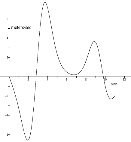
8. Masakazu visited Disneyworld to enjoy a new ride, called the Rocket Sled. In the Rocket Sled, Masakazu was strapped into a car seat, facing forward, with a six-point harness across his chest and shoulders. The car accelerated forward and backward along a long, straight rail. The graph below shows Masakazu's velocity in relation to the number of seconds since the Rocket Sled began moving.
   

1. During what intervals of time, approximately, did Masakazu feel pressure on his back? Explain.
2. During what intervals of time, approximately, did Masakazu feel pressure on his chest? Explain.
3. When, approximately, did Masakazu feel the greatest pressure on his chest? The greatest pressure on his back? Explain.
9. Stanford Oil maintains large holding tanks at the Newark, NJ port. Ships pump oil into holding tanks; pumps drain oil from the tanks into oil trucks, which then deliver oil to utility companies in the region. Sometimes a ship pumps oil into a holding tank while pumps fill oil trucks.

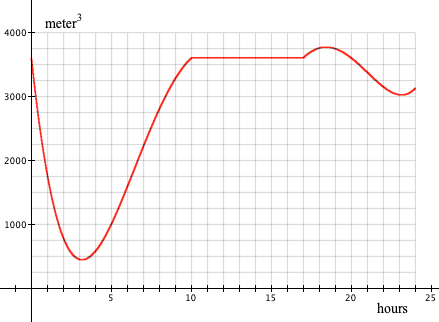
   The graph below shows the volume of accumulated oil in a holding tank over a 24-hour period. Answer questions (a)-(d) with approximate values.

   

   1. Over what intervals of time was a ship pumping oil into the holding tank at a greater rate than oil was being pumped into trucks?
   2. Over what intervals of time was a ship pumping oil into the holding tank at the same rate as oil was being pumped into trucks?
   3. Over what intervals of time was a ship pumping oil into the holding tank at smaller rate than oil was being pumped into trucks?
   4. At what moment in time was the difference between the ship's pumping rate and the trucks' pumping rate greatest? Least?