Section 7.1
Properties of Rate of Change Functions and What They Tell Us
Review and Introduction
In Chapter 3 we developed the meaning of constant rate of change. In Chapter
4 we learned that a function's rate of change at a moment provides useful information about the function's behavior at that moment. In Chapter 6 We learned how to derive an accumulation function's exact rate of change function defined in closed form.
Knowing an accumulation function's rate of change at all moments in an interval provides useful information about the function's behavior over that interval.
Suppose $r_f(k)=c$.
$r_f(k)=c$ means the function f has essentially a constant rate of change of c over a small interval containing $x=k$.
The function f having an essentially constant rate of change over a small interval containing $x=k$ means f is essentially linear over that interval.
f being essentially linear over an interval means $f(x) \doteq r_f(k)(x-k)+f(k)$ for all x in that interval containing $x=k$.
Example 7.1.1
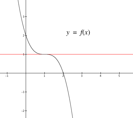
The function f is defined as $f(x)=0.5\sin(3x)$. Therefore, $r_f(x)=1.5\cos(3x)$. Examine the behavior of $y=f(x)$ in relation to $y=r_f(k)(x-k)+f(k)$ at the moment that $x=k=2.45$.
Figure 7.1.1. Examining the behavior of
$f(x)=0.5\sin(3x)$ at the moment that $x=2.45$. The behavior of f is
essentially linear, with $f(x) \doteq r_f(k)(x-k)+f(k)$, over a suitably
small interval containing $k=2.45$.
Reflection 7.1.1. The graph of $y=r_f(k)(x-k)+f(k)$ appears to change slope in the last three zooms. Does it actually change? If not, then why does it appear to change?
Change the definition of f to something other than what it is;
re-define $r_f$ appropriately.
Set the value of k to center on where the function varies most rapidly.
Do as in Figure 7.1.1 to explore whether f is essentially linear over a suitably small interval containing the value of k.
Type ctrl-R to reset GC's graph.
Let $k=n$.
Click "n" on the n-slider. Set the lower bound to -4 and the upper bound to 4. Click OK.
Click the n-slider's play button. Examine the relationship between the sign of $r_f$ and whether the function is increasing or decreasing. What can you say about this relationship?
Do these steps with three different definitions of f.
There are exceptions to when you can use the rate of change function for a function f to conclude something about the behavior of f around a particular value of x. Activity 7.1.2 illustrates this.
Does the value of $r_f(x)$ vary continuously? Explain.
Explore the behavior of f and its linear approximation around $x=1$. What do you notice?
Explain why you cannot say that f is locally linear around $x=1$?
What does this example suggest must be true about a function f and its rate of change over an interval containing $x=a$ in order to say that f is locally linear at the moment that $x=a$? (Hint: Enter the statement $y'=r_f(x')$ in GC.
Recall that the use of
prime in GC just means to display the graph in the right window pane.)
Rate of Change and Behavior of a Function
First, some terminology:
An interval is closed if it contains its endpoints. It is customary to represent a closed interval with brackets, e.g. [2, 3].
An interval is open if it excludes its endpoints. It is customary to represent an open interval with parentheses, e.g. (2, 3).
You must rely on context to distinguish between (2,3)
as a coordinate pair and (2,3) as an open interval.
Let g be a function defined over a closed interval I.
g is increasing over I if for all u and v in I, $g(u) \lt g(v)$ whenever $u \lt v$.Note
g is decreasing over I if for all u and v in I, $g(u) \gt g(v)$ whenever $u \lt v$.
g has a maximum value in I at x
= kif for all x in I, $x \neq k, g(x) \lt g(k)$.
g has a minimum value in I at x
= kif for all x in I, $x \neq k, g(x) \gt g(k)$.
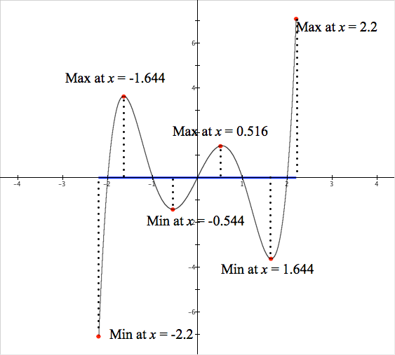
Figure 7.1.2. A function f defined over the closed interval [-2.2, 2.2].
It has minima at $x=-2.2, x=-0.544,\text{and }x=1.644$. It has maxima at
$x=-1.644, x=0.516,\text{and }x=2.2$. The function f would not
have extrema at -2.2 and 2.2 were it defined over the open interval (-2.2,
2.2) because -2.2 and 2.2 would not be in the domain of f's independent
variable.
You saw in Activities 7.1.1 and 7.1.2 that when a function f has a rate of change at the moment $x=k$ that
f is increasing around $x=k$ when $f'(k) \gt 0$.
f is decreasing around $x=k$ when $f'(k) \lt 0$.
f is essentially constant around $x=k$ when $f'(k)=0$.
Case 1: $f'(k) \gt 0$
If $f'(k) \gt 0$, then f is locally linear with a positive rate of change around $x=k$, so f is increasing around $x=k$.
Case 2: $f'(k) \lt 0$
If $f'(k) \lt 0$, then f is locally linear with a negative rate of change around $x=k$, so f is decreasing around $x=k$.
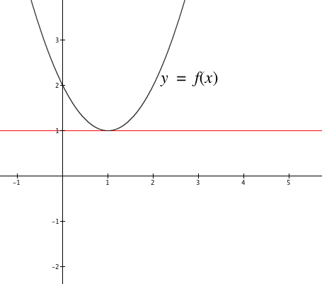
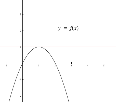
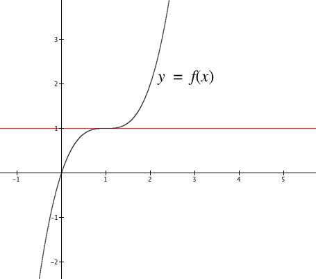
Case 3: $f'(k)=0$
The case of $f'(x)=0$ when $x=k$ is ambiguous with regard to the behavior of f around $x=k$. We know that f is essentially constant around $x=k$ (because $f'(k)=0$), but this can happen in any of four ways. Figure 7.1.2 shows the four possible ways that f can behave around $x=k$ when $f'(k)=0$.
(a) f decreases, then is momentarily constant, then increases. Notice that $r_f(x)$ is negative for $x<1$, then 0 at $x=1$, then positive for $x>1$.
(b) f increases, then is momentarily constant, then decreases. Notice that $r_f(x)$ is positive for $x<1$, then 0 at $x=1$, then negative for $x>1$.
(c) f increases, then is momentarily constant, then increases again. Notice that $r_f(x)$ is positive for $x<1$, then 0 at $x=1$, then positive for $x>1$.
(d) f decreases, then is momentarily constant, then decreases again. Notice that $r_f(x)$ is negative for $x<1$, then 0 at $x=1$, then negative for $x>1$.
Figure 7.1.3. A function can have a rate of change of zero at the
moment x = 1 in four ways.
Extreme Values of a Function (Extrema)
Figure 7.1.3 illustrates a general principle. When $r_f(k)=0$ and $r_f(x)$ changes sign around $x=k$, then f has a maximum or a minimum at $x=k$.
If $r_f(k)=0$ and $r_f(x)$ changes from negative to positive around $x=k$, then f has a minimum value at $x=k$.
If $r_f(k)=0$ and $r_f(x)$ changes from positive to negative around $x=k$, then f has a maximum value at $x=k$.
Activity 7.1.3.
Download this
file. The slider named Function has four values. Each value gives one of the graphs in Figure 7.1.3.
Observe the value (including the sign) of $r_f(n)$ as n increases in value. Is it consistent with the boxed statements immediately above?
Increase the value of Function by one and repeat.
We cannot say that all minima or maxima occur when $f'(k)=0$. Figure
7.1.2 gives an example. A minimum occurs at $x=-2.2$ and a maximum occurs at $x=2.2$ even though neither $f'(-2.2)$ nor $f'(2.2)$ are zero.
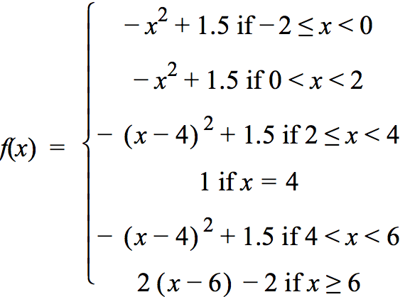
Another instance where an extremum might occur at $x=k$ and $f'(k)$ is undefined. $f'(k)$ can be undefined for a number of reasons, including when $f(k)$ is undefined, when the function is discontinuous at $x=k$ or when $f'(k)$ is undefined because f has a cusp at $x=k$. These cases are shown in Figure 7.1.4.
Figure 7.1.4. The function f is defined for all $x \ge 2$ except
$x=0$. It has a min at x=-2, 2, and 4, but no max at any value of x.
Reflection 7.1.2. Justify each statement in
Figure 7.1.4. For example, explain why f has neither a min nor a max at $x=0$ and $x=6$, and explain how f has a min at $x=2$ and a min at $x=4$ even though $r_f(2)$ and $r_f(4)$ are not zero.
Endpoints of an interval over which f is defined and values of x where $r_f(x)=0$ or $r_f(x)$ is undefined are called critical values of x.
A function defined over an interval I can have a maximum or a minimum only at a critical value of its independent variable.
If $x=k$ is a critical value of x, then you must examine the intervals to the left and right of $x=k$ to see whether they are open or closed at $x=k$.
If an interval is closed (i.e., k is an endpoint of one of those intervals), then a max or min can occur at $x=k$.
If both intervals are open (i.e., k is not in either interval), then f can have a max or min at $x=k$ if it is defined at $x=k$.
f cannot have a max or min at $x=k$ if f is undefined at $x=k$.
Figure 7.1.4 illustrates that you cannot conclude that $f(x)$ is a minimum or a maximum just because $x=k$ is a critical value of x. You must examine the function's behavior around $x=k$.
Global versus Local Extrema
Extrema of a function f can classified as global or local. Suppose a function g is defined over an interval I (which could be all real numbers).
If g has a maximum at $x=k$ and $g(k) \gt g(x)$ for all x in I, $x \neq k$, then $g(k)$ is a global
maximum for g in the interval I.
If g has a maximum at $x=k$ and $g(k)$ is not a global maximum, then $g(k)$ is a local maximum for g in the interval I.
If g has a minimum at $x=k$ and $g(k) \lt g(x)$ for all x in I, $x \neq k$, then $g(k)$ is a global
minimum for g in the interval I.
If g has a minimum at $x=k$ and $g(k)$ is not a global minimum, then $g(k)$ is a local minimum for g in the interval I.
Reflection 7.1.3. Figure 7.1.2 is repeated below. State whether each extremum is global or local over the closed interval $[-2.2,2.2]$? State whether each extremum is global or local over the open interval $(-2.2,2.2)$?
Exercise Set 7.1
Explain why the function f in Figure
7.1.4 (defined over the interval $x \ge -2$) has neither a global maximum nor a global minimum.
Explain, in your own words, the conditions that are necessary for an accumulation function to have:
A global maximum at $x=k$.
A global minimum at $x=k$
No local extremum anywhere in an interval.
A minimum at $x=k$.
A maximum at $x=k$.
Let f be a function and let c be a value in the domain of f. List the ways in which $f'(c)$ can fail to exist.
A student in a previous calculus class made the following statements. Say whether each statement is true or false. If you say "true", then justify your answer. If you say "false", then give an example to show that the statement is false.
The function $f(x)=1/x$ has a global maximum on the interval (0, 1].
All global maxima or global minima occur at a critical value or at an interval's endpoint.
If f is a continuous function, and $f'(c)$ does not exist, then f has neither a maximum nor a minimum at $x=c$.
For questions 5-9.
Bill threw a ball into the air. The ball reached its peak height at 4.1 seconds and hit the ground after 10.5 seconds. The value of $g(t)$ gives the ball's height above ground in meters t seconds after Bill threw the ball.
Each of Part (a) to (d) might be answerable or not. If it can be answered, do so; if it cannot be answered with the given information, explain why.
$g(1)=3.2$. What information does this tell us about the ball’s height?
$g(1)=3.2$. What information does this tell us about how fast the ball’s height is varying at 1 second?
$g’(2) = 1.6$. What can this tell us about how high the ball is at 2 seconds?
$g’(2) = 1.6$. What can this tell us about how fast the ball’s height is varying at 2 seconds?
$g(3.7)=4.5$ and $g’(3.7)=0.2$.
Estimate how high the ball is at 3.77 seconds and explain your work in 2-3 sentences.
Sketch a graph of g for the interval $t=3.63$ to $t=3.77$.
Write an equation to describe your sketch for 2b.
What did you assume about the ROC of g for that interval? How is your assumption reflected in your graph?
Is g increasing, decreasing, or neither over the interval (3.63, 3.77)?
During what intervals of time is:
g increasing? Why?
g decreasing? Why?
During what intervals of time is:
g’ increasing? Why?
g’ decreasing? Why?
For what value(s) of t is:
g(t) = 0? Why?
g’(t) = 0? Why?
For each of (a) and (b), define a rate of change function $r_g$ so that its accumulation function g satisfies the following conditions. Then use GC to graph $r_g$ in the left pane and g in the right pane. On a printout of the two, highlight the features on $r_g$'s graph that correspond to the given properties on g.
On the interval [0,2], $r_g(0.5)=0, r_g(1)=0$, g has a global maximum at $x=2$, g has a global minimum at $x=0$, and g has a local minimum at $x=1$.
On the interval [-1,2], $r_g(0)=r_g(1)=r_g(2)=0$, g has a global maximum at $x=-1$, g has neither min nor max at $x=1$, and g has a global minimum at $x=2$.
Henry tried to communicate to Sandra a relationship between y and x that he called f. Henry, playfully, described this relationship to Sandra via text message, giving her information about $f’$ instead of f. Here is what Henry told Sandra: $f’(2)=1, f’(4)=-2,$ and f’ has local maximums at x=-1 and x=3 and a global maximum at x=7.
Sandra replied, "Not enough info to get your exact graph!"
Sketch 3 different graphs for f that fit these criteria.
Sketch 3 different graphs for f’ that fit these criteria.
Henry texted Sandra again about a new function g, and told her only that $g(3)=0.7$ and $g’(3)=5.6$. This is enough information to write the definition for a linear function (call it h) that is a good approximation of $g(x)$ from $x=2.9$ to $x=3.1$. Sandra replied, "Got it! Your linear function is ... " and she was correct. Write Sandra's definition of h.
Some textbooks say that a function f is decreasing over an interval $[a,b]$ if for all values of x and y in $[a,b]$, $f(x) \ge f(y)$ whenever $x \lt y$.
The animation below shows how the value of tan(x) varies as the value of x (in radians) varies.
Answer this question based solely on the graph of $y=\tan(x)$: "Does the value of tan(x) ever decrease as the value of x increases?"
Does the tangent function's rate of change function ever have a negative value? What does this say about whether the value of tan(x) ever decreases?
If your answer to (a) is "Yes" and your answer to (b) is "No", then you have experienced a contradiction. Resolve the contradiction by doing either of the following. Explain your answer.
Revise the definition of a decreasing function given at the beginning of this exercise (explain your revision), or
Revise your understanding of the definition of a decreasing function given at the beginning of this exercise. Explain your revised understanding and how your understanding changed.
The function v is defined as $v(x)=\sum\limits_{k=0}^{10} 2^{-k}\sin\left(2^kx\right).$
Use GC to estimate the value of $v(7)$. How did GC calculate this value?
Use GC to estimate the value of $r_v(7)$. What is the meaning of $r_v(7)$?
The function j is defined as $$j(x) = \left\lbrace\begin{align} &\dfrac{\cos(x)-1}{x} &\text{ if }x \neq 0 \\ &0 &\text{ if }x = 0 \end{align}\right.$$.
What is $j'(0)$?
According to your answer to (a), what should the graph of j look like around $x=0$?
Graph the function j in GC. Zoom in on the graph around $x=0$. Does it look as you expected? If not, why?
In GC, define the function r as $$r(x)=\frac{j(x+0.001)-j(x)}{0.001}.$$Use GC to evaluate $r(0)$.
Does the value of $r(0)$ make sense relative to the graph of $y=j(x)$? Why?
Does the value of $r(0)$ make sense relative to the definition of
j? Why?
What do you now think is the value of $j'(0)$? Explain.
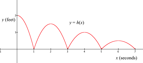
A steel ball bearing is dropped vertically from a height of 2 feet above a concrete floor. The ball bounces vertically repeatedly. Values of the function h give the bearing's height above the ground at each moment in time during the first 7 seconds after it was released. The graph of $y=h(x)$ is shown below. Assume that the bearing varies direction instantaneously each time it bounces.
At what values of x is $h(x)$ defined?
At what values of x is $r_h(x)$ defined?
At what moments in time does the bearing's height have a local maximum? A local minimum?
Does h have a global maximum? A global minimum? Explain.
At what moments in time does the bearing's height have a rate of change of 0?
Over what intervals of time is the bearing's height increasing? Decreasing?
Over what intervals of time is the bearing's rate of change of height with respect to time increasing? Decreasing?
Approximately how far is the ball from its initial position at $t=4$ seconds?
A ball suspended by a 10-foot long rubber cord is at rest. It is given a sudden push downward; the cord stretches, then retracts, pulling the ball upward. The ball bobs up and down with time. (See the animation, below). The ball's displacement from rest is given by the function d, defined as $$d(t)=-e^{-0.0625t}4\sin(t), 0≤t≤18$$where d(t) is in feet and t is in seconds since the ball was pushed.
At what moments during the first 18 seconds does the ball's displacement reach a local minimum? A local maximum?
Does the ball's displacement from rest have a global maximum? A global minimum?
Over what intervals of time is the displacement's rate of change with respect to time increasing? Decreasing?
The amount of water in a Phoenix water tower varies according to time of day. The function w gives the amount of water (in thousands of gallons) in the tank t hours after noon on March 1, 2011. The graph of $y=r_w(t)$ is displayed below.
What does it mean that the point (0.9, 2.4) is on the graph of $y=r_w(t)$?
What is the unit of $r_w(t)$?
Over what period(s) of time was the amount of water in the tank increasing? Explain.
At approximately what time of day was the tank fullest? Explain.