Section 6.3
A Garden of Exact Rate of Change Functions

6.3.1 Motivation

Here’s a secret: GC uses approximations to compute $\displaystyle{\int_a^x r_f(t)dt}$ for any function $r_f$.

When GC integrates a function over a large domain it can be quite inaccurate because it always uses 512 subintervals. So when GC computes $$\int_0^{1024} r_f(t)dt$$ it uses subintervals of size 2, which could produce a highly inaccurate result if $r_f$ varies dramatically within those subintervals.

However, Section 6.2 gave us the insight that we can compute an integral of a function $r_f$ exactly whenever we know an accumulation function f in closed form that has $r_f$ as its rate of change function.

This fact bears repeating.

Whenever we know a closed form representation of a function f that that has $r_f$ as its exact rate of change function, we can use the closed form representation of f to compute $\int_a^x r_f(t)dt$ exactly, namely $$\int_a^x r_f(t)dt=f(x)-f(a).$$We do not need an approximate accumulation function when we can represent the exact integral in closed form.

This fact motivates us to derive rate of change functions in closed form from accumulation functions in closed form. As we derive more accumulation-rate pairs in closed form, our ability to  compute integrals exactly will grow.

A general remark will be helpful in all the remaining sections.

When $0<h<1$ and n is a positive integer, $h^{n+k}$ is smaller than $h^n$ by a factor of $h^k.$ If $h=0.01,$ then $0.01^{15}$ is smaller than $0.01^{10}$ by a factor of $0.01^5,$ or $\left(\frac{1}{100}\right)^5.$ Stated generally, for $0<h<1$, as $h$ becomes small, $h^n$ becomes even smaller, and becomes smaller orders of magnitude more rapidly as the value of n increases.

Practice

Here is a sheet of practice problems. Examine it repeatedly during your study of this chapter for problems that you can solve with methods you have learned up to the moment that you are examining the sheet. You will learn a method for checking your work graphically. Use it.

6.3.2 Derived Rate of Change Function of a Constant Function and a Constant Times a Function

Intuitively, if a quantity has the same measure at every moment of its independent variable, then its value is not varying and its rate of change is 0. More formally, for $h\ne0$

$$\color{red}{\text{(Eq. 6.3.1)}}\qquad \begin{align} f(x)&=c\\[1ex] r(x)&=\frac{f(x+h)-f(x)}{h}\\[1ex] &=\frac{c-c}{h}\\[1ex] &=0\\[1ex]r_f(x)&=0 \end{align}$$

In regard to recovering f from its rate of change function, we have the seemingly odd result that when $f(x)=c$, $\int_a^x r_f(t)dt=0$, not c.

This oddity is only apparent. If you think of f as an accumulation function and $\int_a^x r_f(t)dt$ as f’s net accumulation from a to x, nothing additional has accumulated. Put another way, we know that $f(x) = c$ for some constant c when $r_f(x)=0$ for all x, so by the FTC, $\int_a^x 0dt = f(x)-f(a) = c-c=0$.

When $g(x)=c \cdot f(x)$, where c is a constant, then
$$\begin{align} r_g(x) & = \frac{g(x+h)-g(x)}{h} \\[1ex] & = \frac{c \cdot (f(x+h)-f(x))}{h} \\[1ex] & = c \cdot \frac {f(x+h)-f(x)} {h} \\[1ex] & = c \cdot r_f(x) \\[1ex] \end{align} $$
Therefore, by the FTC, $ \int_a^x c r_f(t)dt = c \int_a^x r_f(t)dt = c (f(x)-f(a))$

6.3.3 Derived Rate of Change Functions for Power Functions

Let $f(x)=cx^n$, n a positive integer and $c≠0$. We want $r_f$, f's exact rate of change function, in closed form.

We’ll start with $n=3$ and use that to generalize to arbitrary integer values of $n≥0$. We’ll also start with the approximate rate of change function and get the exact rate of change function by making the value of h so small that $h \doteq 0$.

If our derivation is correct, then the graphs of the open form and closed form rate of change functions should coincide, and the graphs of the open form and closed form integrals should coincide.

Example:

$$\begin{align} f(x)&=4x^3\\[1ex] r(x)&=\frac{f(x+h)-f(x)}{h}\\[1ex] &=\frac{4(x+h)^3-4x^3}{h}\\[1ex] &=\frac{4\left(x^3+3x^2h+3xh^2+h^2\right)-4x^3}{h}\\[1ex] &=\frac{4\cdot x^2h+4\cdot 3xh^2+4h^3}{h}\\[1ex] &=4\cdot x^2+4\cdot 3xh + 4h^2\\[1ex] r_f(x)&\doteq 4\cdot 3x^2 \text{ when }h \doteq 0 \end{align}$$

Generalization:

Check Example:

Let $f(x)=4x^3$. Use GC to see whether the graph of $y=12x^2$ coincides with the graph of $y=\dfrac{f(x+h)-f(x)}{h}$ when $h=0.0001$. What does this tell you?

Use GC to see whether the graphs of $y=\int_a^x 12t^2dt$ and $y=4x^3-4a^3$ coincide. What does this tell you?

Check Generalization:

Let $f(x)=cx^n$. Use GC to see whether the graph of $y = cnx^{n-1}$ coincides with the graph of $y=\dfrac{f(x+h)-f(x)}{h}$ when $h=0.0001$ and n is any arbitrary value.

What does this tell  you?

Use GC to see whether the graphs of  $\displaystyle{y=\int_a^x cnt^{n-1}dt}$ and $y=c(x^n-a^n)$ coincide for arbitrary values of c and n. What does this tell you? In what way is this result an instance of the FTC?

Applications

Let $g(x)=4$. What is $\int_a^x g(t)dt$?

Rewrite g as $g(x)=4 \cdot 1x^0$. Then $\int_a^x g(t)dt = \int_a^x 4 \cdot 1t^0dt = 4(x^1-a^1)$.

Reflection 6.3.1. Think of what $g(x)=4$ means when g is a rate of change function. Give a concrete example that illustrates how it make sense that $\int_a^x 4dt = 4(x-a)$.

Let $g(x)=7x^3$. What is $\int_a^x g(t)dt$ in closed form?

Were $g$ defined as $g(x)=4x^3$ we would know by the FTC that $\int_a^x 4t^3 dt = x^4 - a^4$. But the coefficient of $x^3$ is 7, not 4. We can adjust for this by noting that $7 = \frac{7}{4} \cdot 4$, so we can write $g(x)=7x^3$ as $g(x)=\frac{7}{4}(4t^3)dt$, so $\int_a^x 7t^3dt = \int_a^x \frac{7}{4}(4t^3)dt=\frac{7}{4}(x^4-a^4)$.

6.3.4 Derived Rate of Change Functions for Sum Functions

Suppose that you walk away from your friend on a straight sidewalk at 6 km/h and your friend walks away from you at 4 km/h.

Every hour that the two of you walk, you will get 6 km further from him and he will get 4 km further from you. So, the distance between the two of you increases at a rate of $(6 + 4)$ km/h.

In general, if $k(x) = f(x)+g(x)$ and if $r_f$ and $r_g$ exist, then $r_k(x) = r_f(x)+r_g(x)$. We can prove the general statement as follows.

Assume that $k(x) = f(x)+g(x)$ and that $r_f$ and $r_g$ exist for all values of x. Remember that "$\doteq$" means "essentially equal to".

$$\color{red}{\text{(Eq. 6.3.2)}}\qquad \begin{align} k(x)&=f(x)+g(x)\\[1ex] r(x)&=\frac{k(x+h)-k(x)}{h}\\[1ex] &=\frac{(f(x+h)+g(x+h))-(f(x)+g(x))}{h}\\[1ex] &=\frac{(f(x+h)-f(x))+(g(x+h)-g(x))}{h}\\[1ex] &=\frac{(f(x+h)-f(x))}{h} + \frac{(g(x+h)-g(x))}{h}\\[1ex] r_k(x)&\doteq r_f(x) + r_g(x) \text{ when }h \doteq 0 \end{align}$$

Library of ROC/Integral pairs, Version 2

Application

Let $h(x)=5x^2-3x+4$. What is $\displaystyle{\int_a^x h(t)dt}$ in closed form?

Rewrite h as $h(x)=f(x)+g(x)+k(x)$, where $f(x)=5x^2$, $g(x)-3x$, and $k(x)=4$. We can use the FTC to find $\displaystyle{\int_a^x h(t)dt}$ in closed form:

$$\begin{align} \int_a^x h(t)dt &= \int_a^x f(t)dt + \int_a^x g(t)dt +\int_a^x k(t)dt\\[1ex] &= \int_a^x 5t^2dt + \int_a^x -3t^1dt +\int_a^x 4t^0dt\\[1ex] &= \int_a^x \frac{5}{3} \cdot 3t^2dt + \int_a^x -\frac{3}{2} \cdot 2t^1dt +\int_a^x 4t^0dt\\[1ex] &= \frac{5}{3} \int_a^x 3t^2dt - \frac{3}{2}\int_a^x 2t^1dt +4\int_a^x t^0dt\\[1ex] &=\frac{5}{3}(x^3-a^3)-\frac{3}{2}(x^2-a^2)+4(x-a)\end{align}$$

Notice in this last example that we changed, for example, $\int_a^x5t^2dt$ to the equivalent statement $\int_a^x \frac{5}{3}\cdot 3t^2dt$.

We then rewrote the second statement as $\frac{5}{3}\int_a^x 3t^2dt$.

This sleight of hand was simply to put the integral into a form that makes it easier to apply the FTC, namely that $\displaystyle{\int_a^x 3t^2dt=x^3-a^3}$.

Exercise Set 6.3.4

1. Given that $f(x)=\dfrac{1}{2}x^3-2x+4$, use $r(x)=\dfrac{f(x+h)-f(x)}{h}$ to derive f’s exact rate of change function, $r_f$, expressed in closed form. Check your derivation by graphing it along with the graph of $y=r(x)$, with $h=0.001$.


2. Find the exact rate of change function, $r_h$, in closed form, for each function h defined below. Use GC to check your answers by graphing $y=r(x)$ and $y=r_h(x)$.


1. $h(x)=5x^4-10x+2$


2. $h(x)=\dfrac{5}{3}x^2-1$


3. $h(x)=\dfrac{1}{4}x^6 + \dfrac{1}{3}x^3 - x^4$


3. Write $\int_a^x h(t)dt$ in closed form for each function h in Exercise 2. Use GC to check your answers.


4. In one kind of chemical reaction two separate substances combine to form a third substance.  The function g, defined as $g(t)=18t-3t^2$, gives the accumulated amount of the third substance t minutes since the reaction began.


1. What is $r_g$, g’s exact rate of change function, in closed form?


2. At what rate is the third substance being produced at the moment that 2 minutes have passed?  At the moment that 4 minutes have passed?


3. Describe in your own words what (b) tells you about the production of the third substance at the 2-minute and 4-minute mark. (adapted from Kline, p. 35)


5. Angry Birds is a popular game for mobile devices.  The goal of Angry Birds is to use a slingshot to shoot angry birds at green pigs.  This goal is achieved by knocking down walls that protect the pigs.  The path of a red bird that is fired from a slingshot can be modeled by the function h, defined as $h(t)=-16t^2+48t+8$, where $h(t)$ is the height of the bird (in meters) off the ground, and t is the number of seconds that have elapsed since the slingshot was released.






1. What is the exact rate of change function, $r_h$, whose values give the rate at which the red bird’s height varies at each moment in time?


2. What restrictions should we place on our dependent and independent variables?  Why?


3. What is the maximum height that the red bird will reach?  Use your rate of change function to justify this solution.


4. Blue birds fly into the screen from the left side. We know that a blue bird’s rate of change of distance from the ground at any moment is modeled by $r_f(t)=-32t+20$ m/s, where t is the number of seconds since it entered the screen.  Determine the blue bird’s change in height between 0.5 seconds and 1 seconds assuming that it entered the screen 10 meters above the ground.




5. Compare the blue bird’s maximum height to the red bird’s maximum height.


6. The binomial coefficients, denoted ${n \choose k}$ where $${n \choose k} = \frac{n!}{(n-k)!k!},$$ are the coefficients of the powers of x when $(x+1)^n$ is expanded.  That is,
   
   $$\begin{align} (x+1)^n & = {n \choose 0}x^0 \cdot 1^n + {n \choose 1}x^1 \cdot 1^{n-1} + {n \choose 2}x^2 \cdot 1^{n-2} + ... + {n \choose {n-1}} x^{n-1} \cdot 1^1 + {n \choose n}x^n \cdot 1^0 \\[1ex] & = {n \choose 0}x^0 + {n \choose 1}x^1 + {n \choose 2}x^2 + ... + {n \choose {n-1}} x^{n-1} + {n \choose n}x^n \\[1ex] \end{align}$$
   
   In Section 6.2 we found that when $f(x)=(x+1)^n,  r_f(x) = n(x+1)^{n-1}.$ Use the expansion of $(x+1)^n$ given above to find another representation of the exact rate of change of $f(x)=(x+1)^n$ with respect to x. Keep in mind that all terms of the form ${n \choose k}$ are constants in the expansion of $(x+1)^n$.


7. Explain why it is reasonable that $f(x)=x^n+a$ and $g(x)=x^n$ should have the same rate exact rate of change function. Consider the relationship between the graphs of f and g.


8. In Section 3.13, Exercise 5, we presented a scenario where two baseball players were running from first to second base and from second to third base, respectively. Player 1 ran at 18 $\mathrm{\frac{ft}{sec}}$.


1. What does $\int_0^5 18dt$ represent in this situation?  Evaluate this integral as part of your explanation.


2. Derive the exact rate of change function for $\int_a^x 18dt$ and explain what it means in regard to Player 1.

6.3.5 Derived Rate of Change Functions for Composite Functions

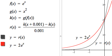
Suppose that k is a composite function such that $k(x)=g(f(x))$ for functions $f$ and $g$. Suppose further that $f$ and $g$ have rate of change functions $r_f$ and $r_g$.

It seems intuitive to think that $r_k$, the exact rate of change function for k, would be $r_k(x)=r_g(f(x))$.

Were this true, then for $k(x)=\left(e^x\right)^2$, $r_k$ would be $r_k(x)=2\left(e^x\right)^1$.

Figure 6.3.1 shows that our intuition is wrong. The graph of r, which we know should be a reasonably good approximation to k’s exact rate of change function, is not even close to the graph of $y=2e^x$. So $r_k(x)≠2e^x$ when $k(x)=(e^x)^2$.

  

Rate of change magnifies variations

A useful way to think about the composite function k where $k(x)=g(f(x))$ is to remind ourselves that $f(x)$ is the argument to g, not g’s independent variable.

If we were to say $u=f(x)$ and ask about the rate of change of g with respect to u, then $r_k(u)$ would indeed be 2u.

But u is varying at a rate of its own with respect to x, so it is as if variations in x get magnified by f, and then variations in f get magnified by g.

Let’s go further with thinking of rate of change as magnification.

Suppose you have two lenses, f and g, and that f magnifies objects to make them appear 2 times as large, and g magnifies objects to make them appear 3 times as large.

• Think of holding g over a rubber stick. The stick, to your eye, is magnified 3 times its original length.
• Now slip lens f between lens g and the stick. Lens f magnifies the stick by a factor of 2. Lens g magnifies the magnified image it receives from lens f by a factor of 3.
• So in the image you see, the stick has been magnified twice, so its total magnification is by a factor of $3 \cdot 2$.

Here is where the idea of rate of change as magnification comes in.

• Call the length of the stick x. Now imagine that you stretch the stick to make it a little longer—$dx$ longer.
• Lens f magnifies that change so that the change of $dx$ in x is magnified in f’s image to be 2$dx$. The rate of change of f’s image with respect to variations in x is 2.
• Lens g magnifies the magnified change by a factor of 3, so in the final image the change of $dx$ in the stick’s length is magnified to be twice as large by f and then three times as large by g.
• The change of $dx$ in x becomes a change of $3 \cdot 2 dx$ in the image produced by g. That is, if we call the length of the the stick in g’s image y, then $dy=3 \cdot 2 dx$. The rate of change of the image produced by $g(f(x))$ is 6 with respect to variations in x.

So it is with functions in general: variations in x are magnified by $r_f$, and variations in f are magnified by $r_g$. When $k(x)=g(f(x))$, we have $r_k(x)=r_g(f(x))r_f(x)$. This chain of magnifications is shown in Figure 6.3.2.

Note that Figure 6.3.2 shows three number lines, vertically. The first is the x number line, the second is the f(x) number line, and the third is the k(x) = g(f(x)) number line. In all three, up is positive and down is negative.

Figure 6.3.2 also shows differentials in each of x, f(x), and $k(x)=g(f(x))$. The black arrows show how the differentials are related.

Figure 6.3.2 shows two views of the chain of variations in x, f(x), and g(f(x).

• The first phase of the animation shows the relationship among differentials (variations) in x, $f(x)$, and $g(f(x))$.
• The differential (variation) in x (i.e., dx) is magnified by $r_f(x)$ to get a change in f (df),
• The differential df is magnified by $r_g(f(x))$ to get dk, the differential in k.
• Keep in mind that magnifications can be greater than 1 or less than 1, and that magnifications can be negative (giving a flipped image).
• Also keep in mind that it is variations (differentials) that are magnified, not the value of x or the value of $f(x)$.
• The second phase of the animation shows directly how differentials in x are related to differentials in $k(x)=g(f(x))$.

The equation $r_k(x)=r_g(f(x))r_f(x)$, being a chain of magnifications, is called the chain rule.

Application

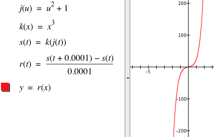
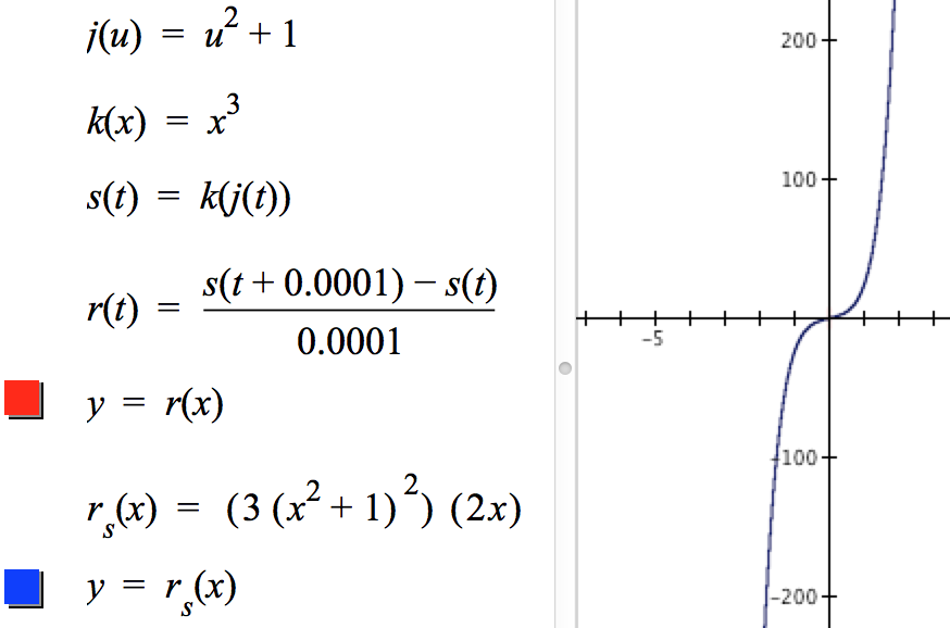
Let the functions j, k, and s be defined as $j(u)=u^2+1$, $k(x)=x^3$, and $s(t)=k(j(t))$. According to Version 2 of our Library, $r_j(u)=2u$ and $r_k(x)=3x^2$. Therefore, by the general rule that $r_s(x)=r_k(j(x))r_j(x)$, we have that $r_s(x)=(3(x^2+1)^2)(2x)$.

Let’s check this in GC.

Figure 6.3.3 starts with the closed form accumulation functions $j(u)=u^2+1$, $k(x)=x^3$, and $s(t)=k(j(t))$. The left side also shows GC’s graph of s’s approximate rate of change function, r.

The right graph shows that GC’s graph of our derived function $r_s$ coincides with the graph of r.

Since we trust GC’s graph of r to be a close approximation of s’s actual rate of change function’s graph, Figure 6.3.3’s right image supports our analysis.

(a)

(b)

 
Figure 6.3.3. Testing ROC of composite function. The graph of $y=r(x)$ appears to coincide with the graph of $y=r_s(x)$.

Application: Using the Chain Rule to extend the Power Rule

We derived the general rate of change function for a power function whose exponent is a natural number, namely $r_f(x)=nx^{n-1}$ when $f(x)=x^n$.

We will use the chain rule together with the fact that $x^{-n}=\left(x^{-1}\right)^n$ to extend the power rule to the case of any accumulation function that is raised to a negative integer power.

To do this we must first derive the rate of change function for $f(x)=x^{-1}$, or $f(x)=\frac{1}{x}$. We do this in Equation 6.3.2.

$$\color{red}{\text{(Eq. 6.3.2)}}\qquad \begin{align}
f(x)&=\frac{1}{x}\\[1ex]
r(x)&=\frac{f(x+h)-f(x)}{h}\\[1ex]
&=\frac{\left(\dfrac{1}{x+h}\right)-\left(\dfrac{1}{x}\right)}{h}\\[1ex]
&=\frac{\dfrac{x-(x+h)}{x(x+h)}}{h}\\[1ex]
&=\frac{x-x-h}{hx(x+h)}\\[1ex]
&=\frac{-h}{hx(x+h)}\\[1ex]
&=\frac{-1}{x(x+h)}\\[1ex]
r_f(x)&\doteq \frac{-1}{x^2}
\end{align}$$

Now let h be defined as $h(x)=x^{-n}$, n a positive integer. We can rewrite h as $h(x)=f(g(x))$, where $f(x)=x^n$ and $g(x)=x^{-1}$. By the chain rule, we have

In Equation 6.3.3, we used the chain rule to generalize the power rule to $r_h(x)=-nx^{-n-1}$ when $h(x)=x^{-n}$ for positive integers $n$. Therefore, $r_h(x)=nx^{n-1}$ when $h(x)=x^n$ whether $n$ is negative or positive.

Using the chain rule effectively

Using the chain rule effectively requires more than remembering it. The primary difficulty in using it effectively is recognizing that a function definition entails a composition of functions. There are two ways of thinking (WOT) that can help.

Another question you will certainly have is, "When should I use the chain rule?". The answer to this question is, "Always!!". You can never go wrong by always using the chain rule. The worst that can happen is that your last rate of change function is 1, just like the example in WOT #2, above.

Exercise Set 6.3.5a

1. This exercise is designed to let you practice WOT #1 above. Substitute an expression for x and then apply the chain rule. Use GC to check your answer. Keep in mind that you will not check your derived rate function against the approximate rate function for the function as given, but against the approximate rate function for your composite function.
   
   For example: In (a), substitute $2x^2+1$ for x, getting $f(x) = (2x^2+1)^5$. Apply the chain rule to get the derived function $r_f(x)=5(2x^2+1)^4(4x)$. Check your answer by graphing your derived function and the graph of r defined as $r(x)=\frac{f(x+0.0001)-f(x)}{0.0001}$ (or using g and p as appropriate). If the two graphs do not agree, then it is likely that your derived function for the composite function is incorrect.


1. $f(x)=x^5$; $r_f(x)=5x^4$


2. $g(x)=2x^3-4x^{-2}+0.5x-1$; $r_g(x)=6x^2+8x^{-3}+0.5$


3. $p(x)=(2x+1)^3$; $r_p(x)=3(2x+1)^2(2)$


2. This exercise is designed to let you practice WOT #2 (above). Find the exact rate of change function r sub _ (the function name goes in the blank) for each function. Be alert for the possibility that you need to use the chain rule within using the chain rule in deriving r sub _. Use GC to check your answers.


1. $f(x)=(2(x+1)^2-2x-3)^3$


2. $g(x)=(x^4-(2x^2-2x)^{-2})^3+(x^3+2x^2-x-5)^2$


3. $h(x)=(((x^2+1)^3+2x)^2-3x^4)^3$


4. The function j is defined as $j(x)=u(v(r(s(x))))$ for functions u, v, r, and s that each have a rate of change function defined for all values of x. Use the chain rule to define $r_j(x)$.


5. Relate Part d of this exercise to Parts a-c.

Reversing the Chain Rule

Recall from Chapters 4 and 5 that if a function g has a rate of change at a moment for all values of x, then $dy=r_g(x)dx$ for all moments of x, where $r_g(x)$ is the rate of change of g at the moment x.

We can use this relationship between y and x, together with the chain rule, to integrate rate of change functions that would look too messy to handle normally.

Let $g(x)=x^2+1$, and let $h(x)=3(x^2+1)^2 2x$.

Suppose that $h(x)=r_k(x)$ for some function k. If you look closely, you’ll see that  $2x=r_g(x)$, and therefore that $r_k(x)=3(g(x))^2 r_g(x)$.

We know that $\int_a^x r_k(t)dt = k(x)-k(a)$. If we let $w=g(x)$, then $dw=r_g(x)dx$, and therefore:

$$\color{red}{\text{(Eq. 6.3.3a)}}\qquad \begin{align} k(x)-k(a)&=\int_a^x r_k(t)dt\\[1ex] &=\int_a^x (g(t))^2 r_g(t)dt\\[1ex] &=\int_{g(a)}^{g(x)}3w^2dw\\[1ex] &=(g(x))^3-(g(a))^2\\[1ex] &=(x^2+1)^3-(a^2+1)^3 \end{align}$$

Therefore, when $r_k(x)=3(x^2+1)^2 2x$, we get $k(x)=(x^2+1)^3$ by recognizing that $3(x^2+1)^2 2x$ is the rate of change function for a composite function and then reversing the chain rule.

While there were several key moves in Equation 6.3.3a, the most critical one was to adjust the limits of the integral upon substituting w for $g(t)$.

How might we understand the decision to make this adjustment? Like this:

In general, if you recognize that the rate of change function $r_k$ for an unknown function k has the structure $r_k(x)=r_f(g(x))r_g(x)$, and you recognize the functions f and g that have $r_f$ and $r_g$ as their rate of change functions, then:

$$\color{red}{\text{(Eq. 6.3.3b)}}\qquad \begin{align} \int_a^x r_k(t)dt&=k(x)-k(a)\\[1ex] &=f(g(x))-f(g(a))\\[1ex] &\text{and}\\[1ex] \int_a^x r_k(t)dt&=\int_a^x f(g(t))dt\\[1ex] &=\int_{g(a)}^{g(x)}r_f(w)dw\\[1ex] &=f(g(x))-f(g(a)) \end{align}$$

You obtain the same result whether substituting the arguments of k after integrating (in the arguments of k) or before integrating (in the arguments of the integral).

Exercise Set 6.3.5b

Forthcoming.

6.3.6 Other Notations for Derived Rate of Change Functions

We have used the notation $r_f$ (called rate notation) consistently to represent a function f’s exact rate of change function. We did this continually to drive home the point that we are talking about rate of change functions—functions whose values give the rate of change at a moment of another function.

Now that we are deriving rate of change functions, we’ll begin to use other notations: $\frac{d}{dx}$ (called differential notation) and $f'$ (called prime notation). There is a fourth notational system, $D_f$ (called operator notation) that we’ll not use.

Suppose that $f(x)=(x^2+1)^3$. Up to now we represented f’s rate of change function using rate notation as $r_f$. By applying the derivations we have developed we see that $r_f(x)=3(x^2+1)^2(2x)$.

We would write $r_f(x)=3(x^2+1)^2(2x)$ in differential notation as $$\frac{d}{dx}(x^2+1)^3=3(x^2+1)^2(2x).$$Using prime notation, we would write $$f'(x)=3(x^2+1)^2(2x).$$

Advantages and Disadvantages of Each Notational System

Rate Notation

An advantage of rate notation is that we are reminded that the function we are representing is a rate of change function for another function.

Another advantage is that rate notation allows us to represent a rate of change at a moment explicitly, such as $r_f(\sqrt{2})$ to represent $f$'s eact rate of change at the moment $x=2$.

The advantage of rate notation's emphasis on being a function in relation to another function brings a disadvantage with it.

Unlike differential notation, we lose the sense that we are doing something to the accumulation function to derive its rate of change function. One way to represent that we do something to a function f to get its rate of change function $r_f$ is to write $$r_f(x)=\frac{d}{dx}f(x).$$ GC actually would understand the above statement as defining the function $r_f$.

Differential Notation

An advantage of differential notation is that you see the function’s original defining formula in close proximity with the derived function’s formula.

This makes it easier to remember rules, but it also runs the risk that you forget you are finding a rate of change function that stands in relation to an accumulation function.

Differential notation is often used in the context of having defined a function without the use of function notation. If we write $y=(x^2+1)^3$, then we would write $\dfrac{dy}{dx}=3(x^2+1)^2(2x)$ and interpret it as giving us the momentary rate of change of the function defined by $(x^2+1)^3$ at every value of x.

Another advantage to differential notation is that it reminds us that we are talking about differentials in a function’s independent and dependent variables.

A major disadvantage of differential notation is there no easy way to represent the rate of change of a function at, say, $x=2$. We could substitute 2 for x in $3(x^2+1)^2(2x)$, but this is finding the rate of change at $x=2$. This does not represent the rate of change of f at $x=2$.

A conventional way to represent rate of change at the moment $x=a$ using differential notation is $$\left.\frac{dy}{dx}\right|_{x=a}.$$

Another disadvantage of differential notation is it fosters the idea that a function's defining formula is the function itself. We do not name the original function using differential notation nor do we name its derived function. Rather, the focus is to begin with one expression and end with another.

Prime Notation

Prime notation is very similar to rate notation in that it reminds you that the derived function is a function and not the symbolic expression that defines it.

A practical drawback for us of prime notation is GC interprets the prime sign ($’$) as a command to draw a graph in a second graphing pane. To GC, prime notation has nothing to do with rate of change functions.

Using Different Notations for Rate of Change Functions

The chain rule, for example, is expressed differently in the three notational systems.

Let f and g be functions and let h be the composite function defined as $h(x)=g(f(x))$.

• The chain rule in rate notation: $$r_h(x)=r_g(f(x))\cdot r_f(x).$$
• The chain rule in differential notation: $$\frac{dy}{dx}=\frac{dy}{du}\frac{du}{dx}$$where $y=g(f(x))$ and $u=f(x)$.
• The chain rule in prime notation:$$g((f(x)))'=g'(f(x))\cdot f'(x).$$

Keep in mind that all three statements say the same thing about the rate of change function for a composite function.

Do not read the above statements literally (e.g., "dee y dee x equals dee y dee u times dee u dee x"). Instead, read them in terms of what they mean.

• Read the chain rule expressed in rate or prime notation as, "The rate of change of h with respect to x is the rate of change of g with respect to $f(x)$ times the rate of change of f with respect to x".
• Read the chain rule expressed in differential notation as, "The rate of change of y with respect to x is the rate of change of y with respect to u times the rate of change of u with respect to x".

When to Use Particular Notational Systems

• We use rate notation primarily when we emphasize the relationship between an accumulation function and its rate of change function at moments of their independent variable.
• We use differential notation primarily when emphasizing the relationship between a function’s defining formula and the defining formula of its rate of change function.
• We use prime notation interchangeably with rate notation when our emphasis is on the fact that a derivative (derived rate of change function) is a rate of change function for an accumulation function.

Exercise Set 6.3.6

1. Repeat the exercises in Exercise Set 6.3.5a, but produce your work two times, first using differential notation and second using prime notation.

6.3.7 Derived Rate of Change Functions for Trigonometric Functions

Sine and Cosine

Recall from Chapter 2 the meaning of θ and y in $y=\sin(θ)$: θ is the an angle measure in radians and y is a fraction of a circle’s radius. The animation in Figure 6.3.4 shows sin(θ) and cos(θ) varying in relation to θ.

Focus on sin(θ) in relation to θ. Examine where sin(θ) varies faster and slower in relation to variations in the value of θ. Pause the animation and move the playhead manually to get a sense of how sin(θ) varies for equal increments of θ. Then do the same for cos(θ).

Reflection 6.3.3. Over what intervals of length 0.5 radians does $\sin(\theta)$ vary the most? The least?

We can derive closed form representations for f and g defined as $f(x)=\sin(x)$ and $g(x)=\cos(x)$. In doing so, we will use two identities from trigonometry and two new insights into the sine and cosine functions.

The trigonometric identities are $$\sin(u+v)=\sin(u)\cos(v)+\sin(v)\cos(u)$$which is used in the derivation of sine’s rate of change function in Equation 6.3.4, and $$\cos(u+v)=\cos(u)\cos(v)-\sin(u)\sin(v)$$which is used in the derivation of cosine’s rate of change function in Equation 6.3.6.

Let $f(x) = \sin(x)$. We start the derivation of the closed form representation of f’s rate of change function by starting with its approximate rate of change function:

$$\color{red}{\text{(Eq. 6.3.4)}}\qquad\begin{align} r(x)&=\frac{f(x+h)-f(x)}{h}\\[1ex] &=\frac{\sin(x+h)-sin(x)}{h}\\[1ex] &=\frac{(\sin(x)\cos(h)+\sin(h)\cos(x))-\sin(x)}{h}\\[1ex] &=\frac{\sin(x)(\cos(h)-1)+\sin(h)cos(x)}{h}\\[1ex] &=\sin(x)\left(\frac{\cos(h)-1}{h}\right)+\cos(x)\left(\frac{\sin(h)}{h}\right) \end{align}$$

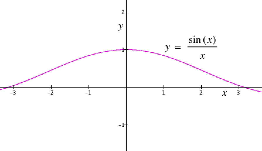
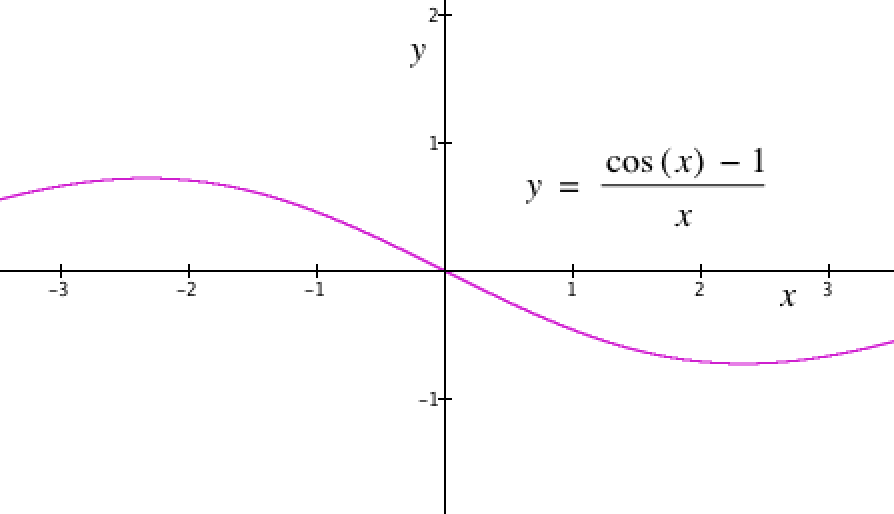
In Equation 6.3.4 we came to line 5, where we need to understand the behavior of $\dfrac{\cos(h)-1}{h}$ and of $\dfrac{\sin(h)}{h}$ for values of h indistinguishable from 0 but not 0. We need to say that $h\neq0$ because neither expression is defined for $h=0$.

Examine the two frames in Figure 6.3.5. Figure 6.3.5a shows GC’s graph of $y=\dfrac{\sin(x)}{x}$. Figure 6.3.5b shows GC’s graph of $y=\dfrac{\cos(x)-1}{x}$. GC’s graph of $y=\dfrac{\sin(x)}{x}$ suggests that $\dfrac{\sin(x)}{x}$ is essentially 1 for values of x near 0. GC’s graph of $y=\dfrac{\cos(x)-1}{x}$ suggests that $\dfrac{\cos(x)-1}{x}$ is essentially 0 for values of x near 0.

(a)

(b)

Figure 6.3.5. $y=\dfrac{\sin(x)}{x}$ and $y=\dfrac{\cos(x)-1}{x}$. Examine their behavior near $x=0$.

If we take as fact that $\dfrac{\sin(x)}{x} \doteq1$ for $h \doteq 0$ and that $\dfrac{\cos(x)-1}{x} \doteq 0$ for $h \doteq 0$, we can write Equation 6.3.5.

$$\color{red}{\text{(Eq. 6.3.5)}}\qquad r_f(x)=\cos(x)\text{ when }f(x)=\sin(x)\text{ and }\int_a^x \cos(t)dt = \sin(x) - \sin(a)$$

From Equation 6.3.5 we can represent the rate of change function for sin(x) in three ways:

• $r_f(x)=\cos(x)$ when $f(x)=\sin(x)$
• $\dfrac{d}{dx}\sin(x)=\cos(x)$
• $f'(x)=\cos(x)$ when $f(x)=\sin(x)$

We can derive a closed form representation of the exact rate of change function for $g(x)=\cos(x)$: Start with an approximate rate of change function, derive a form that allows us to omit terms that involve h by letting h become so small that $h \doteq 0$.

$$\color{red}{\text{(Eq. 6.3.6)}}\qquad \begin{align} r(x)&=\frac{g(x+h)-g(x)}{h}\\[1ex] &=\frac{\cos(x+h)-\cos(x)}{h}\\[1ex] &=\frac{(\cos(x)\cos(h)-\sin(x)\sin(h))-\cos(x)}{h}\\[1ex] &=\frac{\cos(x)(\cos(h)-1)-\sin(x)\sin(h)}{h}\\[1ex] &=\cos(x)\left(\frac{\cos(h)-1}{h}\right)-\sin(x)\left(\frac{\sin(h)}{h}\right)\\[1ex] &\doteq \cos(x)\cdot 0 - \sin(x)\cdot 1\text{ when }h\doteq 0\\[1ex] &\doteq -\sin(x)\text{ when }h\doteq 0 \end{align}$$

From the derivation in Equation 6.3.6 we can conclude that

$$\color{red}{\text{(Eq. 6.3.7)}}\qquad r_g(x)=-\sin(x)\text{ when }g(x)=\cos(x)\\[1ex] \text{ and that }\int_a^x -\sin(t)dt = \cos(x) - \cos(a)$$

From Equation 6.3.6 we can represent the rate of change function for $\cos(x)$ in three ways:

$$\begin{align}r_g(x)&=-\sin(x)\text{ when }g(x)=\cos(x)\\[1ex] \frac{d}{dx}\cos(x) &= -\sin(x)\\[1ex] g'(x)&=-\sin(x)\text{ when }g(x)=\cos(x)\end{align}$$

Because the tangent function is the quotient of sine and cosine functions, we will derive the closed form rate of change function for the tangent function in the next section. It develops the rate of change function for product and quotent functions.

Version 3 of our Library of Rate of Change/Integral pairs is:

Exercise Set 6.3.7

1. Find the exact rate of change function, $r_p(x)$, for each function $p(x)$ shown below. Check your derivation by graphing it along with the graph of p’s approximate rate function.


1. $p(x)=4(3x-8)^6+\sin(4\cos(x^5)+x^3-8)$


2. $p(x)=\cos(-(\sin(x))^2-\cos(x))$


3. $p(x)=\frac{1}{4}(\cos(x^2-4x+8))^8$


2. Suppose you have an exact rate of change function $r(x)=-\sin(x)+\frac{1}{2}\cos(x)+3x^3-8$. Find $\int_a^x r(t)dt$ in closed form.


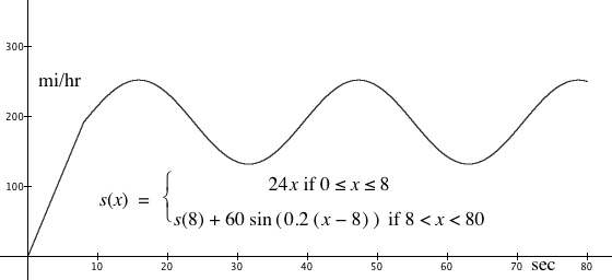
3. Dale Earnhardt, Jr. is trying out a special device that records his speed throughout a NASCAR race.  The figure below shows a display of Dale’s speed, in $\mathrm {\frac{mi}{hr}}$, at each moment during an 80-second period of time.  Dale’s speed is modeled by the function s, which relates Dale’s speed, in $\mathrm {\frac{mi}{hr}}$, to the number of seconds that have elapsed.  






1. What does the function s tell you about what Dale was doing during the first 8 seconds shown on the graph?


2. Explain a likely reason why $s(x)$ is sinusoidal from $x=8$ to $x=80$.


3. A lap at the Charlotte Motor Speedway is 1.5 miles.  Dale’s main competitor, Jeff Gordon, completed 2 laps in the first minute of this 80-second period.  Determine who went farther in the first minute. 


4. Determine $r_s$, the rate of change function for s.  Check your derivation by graphing it along with the graph of s’s approximate rate function.
   
5. Use GC’s graph of $y=r_s(x)$ to state, approximately, the times at which Dale prepared to enter a curve in the track and when he started to come out of the turn, into a straightaway.


6. What does the graph of $y=r_s(x)$ tell you about s as a model of Dale’s speed during this time period?


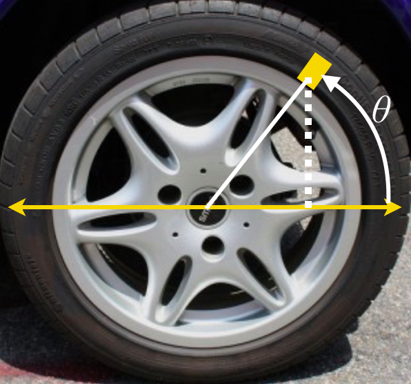
4. A car has a piece of tape on a rear wheel so that we can record the number of radians that the wheel has swept after any amount of time has elapsed.  As the tire rotates, an angle of θ radians is swept out by the piece of tape from the 3 o’clock position. The angle’s measure increases at a rate of 3.4 radians/sec. We started recording the tape’s height from horizontal at a moment when it was 0 cm.




5. Let h be the function such that $h(t)$ represents the vertical height of the tape’s center, in cm, from the horizontal diameter t seconds after recording began. So $h(0)=0$. The tape's center is 25.4 cm from the tire's center. 
1. Determine a rate of change function $r_h$ whose values $r_h(t)$ are the tape’s rate of change of vertical height from the horizontal diameter with respect to the number of seconds that have elapsed. Check your rate of change function by graphing it along with the graph of h’s approximate rate function.


2. At what rate is the tape's vertical height increasing with respect to time at the moment that 235.7 seconds have elapsed?

6.3.8 Derived Rate of Change Functions for Product and Quotient Functions

In this section we will derive the general form of rate of change functions for an accumulation function that is a product of two functions that each have exact rate of change functions.

A quotient function h defined as $$h(x)=\frac{q(x)}{p(x)},\, p(x)\neq 0$$can be expressed as $$h(x)=q(x)(p(x))^{-1}.$$where $(p(x))^{-1}$ means $\dfrac{1}{p(x)}$.

We will therefore treat a quotient of two functions as a product of two functions.

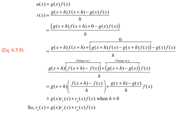
Let u be a product of functions f and g that each have a rate of change function at every moment. Then $u(x)=g(x)f(x)$.

We know that in finding u’s exact rate of change function we will form an approximate rate of change function that has $g(x+h)f(x+h)-g(x)f(x)$ in its numerator. This form, however, is not very helpful for expressing the rate of change function for $u$ in relation to the rate of change functions for $g$ and $f$.

Suppose we were to factor out $g(x+h)$. We could do this if we had $g(x+h)f(x)$ as a term. Well, we can add $g(x+h)f(x)$ and then compensate by subtracting $g(x+h)f(x)$, too, in order to keep the numerator equivalent to $g(x+h)f(x+h)-g(x)f(x)$. This is like adding zero when we add and subtract the same term.

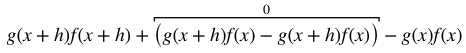
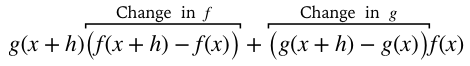
The numerator in its new, equivalent form is

which can be simplified to

which is far more useful as a numerator because it represents both a variation in g and a variation in f.

Equation 6.3.8 employs the trick of adding and subtracting the same term in order to put the approximate rate of change function’s numerator in a more useful form. It ends with the general result that $r_u(x)=g(x)r_f(x)+r_g(x)f(x)$ when u is the product of two functions g and f that each have exact rate of change functions.

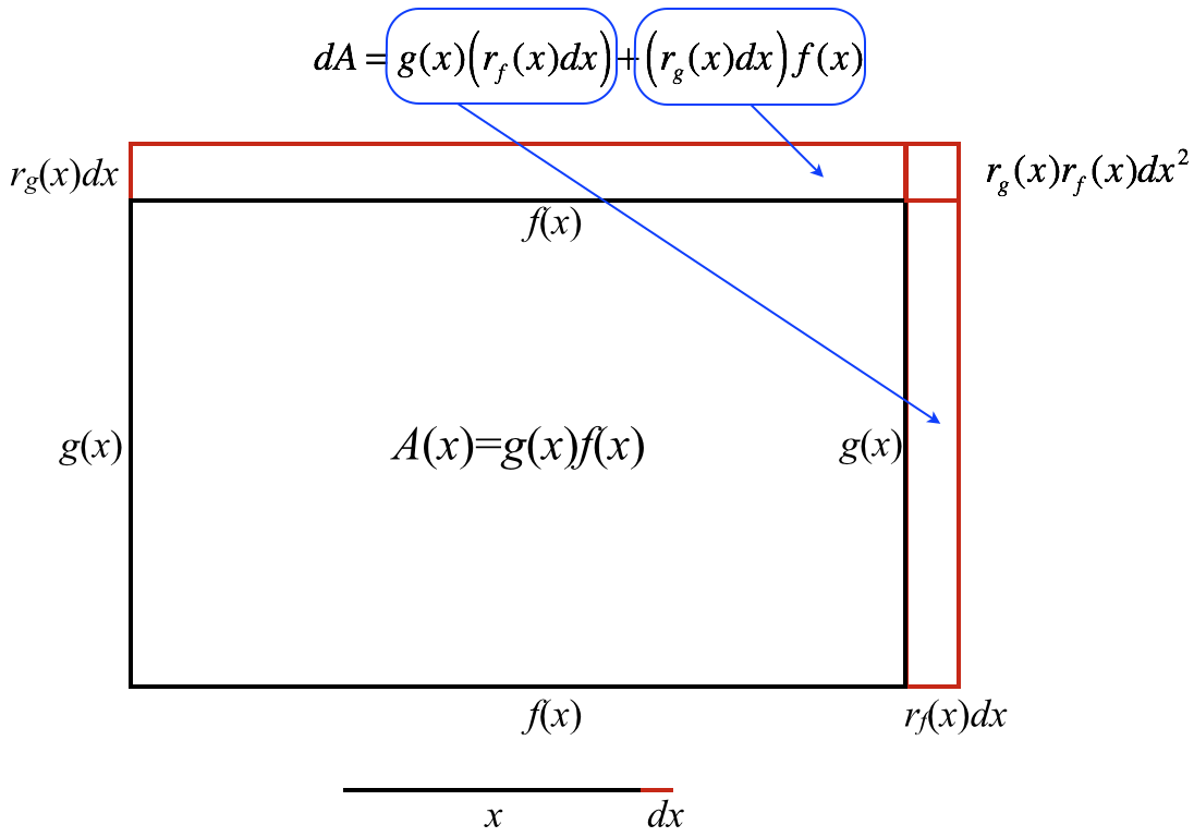
Figure 6.3.6 shows a more intuitive derivation of the rate of change function for a product of functions. It uses area as a model of multiplication. The rectangle has side lengths of $g(x)$ and $f(x)$, so the area function A defined as $A(x)=g(x)f(x)$ gives the rectangle’s area for every value of x. The question is at what rate the area increases when we increase x by dx.

  Figure 6.3.6. Using differentials to derive the rate of change function for a product of functions.

Figure 6.3.6 shows the value of x increasing by a tiny amount dx.

• Since both g and h have exact rate of change functions, they increase at the essentially constant rates $r_g(x)$ and $r_f(x)$ respectively for sufficiently small values of dx.
• Their lengths therefore increase by amounts that are essentially $r_g(x)dx$ and $r_f(x)dx$, respectively.
• The rectangle’s area therefore increases by $g(x)(r_f(x)dx)+(r_g(x)dx)f(x)$ plus $r_g(x)r_f(x)dx^2$
• $r_g(x)r_f(x)dx^2$ is insubstantial given that dx is a tiny increase in x and therefore that $dx^2$ is an order of magnitude smaller.
• Therefore $r_A(x)=g(x)r_f(x)+r_g(x)f(x)$.

We can express the product rule in three ways, using rate, differential, and prime notation:

$$\begin{align} \text{Let }u(x)&=g(x)f(x).\text{ Then:}\\[2ex] r_u(x)&=g(x)r_f(x)+r_g(x)f(x)\\[1.5ex] \frac{d}{dx}u(x)&=g(x)\left(\frac{d}{dx}f(x)\right)+\left(\frac{d}{dx}g(x)\right)f(x)\\[1.5ex] u'(x)&=g(x)f'(x)+g'(x)f(x) \end{align}$$

Application of the Product Rule: The tangent function

The tangent function is defined as $$\tan(x)=\frac{\sin(x)}{\cos(x)}, \cos(x)\neq 0,$$ which can be rewritten as a product: $$\tan(x)=(\sin(x))(\cos(x))^{-1}.$$ We can derive the tangent function’s exact rate of change function by applying the product rule, the power rule, and the chain rule, and using the definition of the secant function as $\sec(x)=\dfrac{1}{\cos(x)}$.

$$\color{red}{\text{(Eq. 6.3.9)}}\qquad \begin{align} \tan(x)&=\frac{\sin(x)}{\cos(x)},\, \cos(x)\neq 0\\[1ex] &=\sin(x)(cos(x))^{-1}\\[2ex] \frac{d}{dx}\tan(x) &=\sin(x)\left(\frac{d}{dx}(\cos(x))^{-1}\right)+\left(\frac{d}{dx}\sin(x)\right)(\cos(x))^{-1}\\[1ex] &=\left(\sin(x)\left(-1(\cos(x))^{-2}(-\sin(x))\right)\right)+(\cos(x))(\cos(x))^{-1}\\[1ex] &=\frac{-(\sin(x))^2}{-(\cos(x))^2}+\frac{\cos(x)}{\cos(x)}\\[1ex] &=\frac{(\sin(x))^2+(\cos(x))^2}{(\cos(x))^2}\\[1ex] &=\frac{1}{(\cos(x))^2}\\[1ex] &=\left(\frac{1}{\cos(x)}\right)^2\\[1ex] &=(\sec(x))^2 \end{align}$$

Therefore, $r_{\tan}(x)=(\sec x)^2$.

We can express the derived rate of change function for $\tan(x)$ in three ways using our three notation schemes:

We can also add our new results to our Library of Rate of Change/Integral Pairs:

Exercise Set 6.3.8

1. Use the product rule to show that $r_g(x)=3$ when $g(x)=3x$.


2. We know that $x^p x^q = x^ {p+q}$. When $k(x)=x^p x^q$ we could simplify $x^p x^q$ to write k as $k(x)=x^{p+q}$ and use the power rule to find that $r_k(x)=(p+q)x^{(p+q)-1}$. Nevertheless, use the product rule to show that $r_k(x)=(p+q)x^{(p+q)-1}$ when $k(x)=x^{p+q}$.


3. Write $$\int_a^x \left(3t^2 \cos(t) + (6t)\sin(t)\right)dt$$ in closed form.


4. A soda company uses 139 $\mathrm{cm}^2$ of aluminum to produce a cylindrical soda can.  Suppose they want to know the best way to make this can (what dimensions it needs for a radius and height) in order to maximize the volume that they can fit into this cylindrical can.


1. Recall the formulas for surface area and volume of a cylinder.


2. Define a function h that represents the cylindrical can’s height as a function of x, the can’s radius (in cm).  (Keep in mind that we have 139 $\mathrm{cm}^2$ of aluminum to use.)


3. Use part (b) to define a function v whose values are the can’s volume in relation to its radius.


4. Define the rate of change function $r_v$. Values of $r_v$ are the exact rate of change of the can’s volume at any moment of its radius as the radius varies from 0 to its maximum value.


5. Determine the value of the radius that produces a can with the largest possible volume.  What is the can’s height when its volume is maximum?

6.3.9 Derived Rate of Change Functions for Functions Defined Implicitly

In Chapter 3, Section 3.10, we distinguished between functions defined explicitly and functions defined implicitly.

In the equation $x^2-xy+y^2=3$ we can envision x being a function of y or y being a function of x over suitably restricted intervals of x and y.

Suppose that we envision x as a function of y. This supposition has the same effect as rewriting $$x^2-xy+y^2=3\text{ as}$$ $$(g(y))^2-g(y)y+y^2=3,$$ where we now interpret "3" as the constant function $f(y)=3$.

We do not know the actual definition of g, nor do we know immediately how y must be restricted so that g is a function. But we can proceed nevertheless with the assumption that g is defined as a function of y and that 3 is a function of y without the definition of g and without knowing ahead of time how y must be restricted.

Assume that g is an accumulation function and that y is its independent variable.

We can then apply what we know about derived rate of change functions to the equation $(g(y))^2-g(y)y+y^2=3$.

Since the left side and right side are equal for all values in the domain of y, the left side will vary at the same rate with respect to y as will the right side.

We can therefore perform the derivation given in Equation 6.3.10.

Print Equation 6.3.10 so that you can write on it as you read the following moves that we made in this derivation.

We:

• Presumed that x can be defined as a function of y (line 2);
• Substituted $g(y)$ for x (line 3);
• Equated the derived functions of the left and right sides of the equation (line 4);
• Applied what we know about derived functions of a sum of functions (line 5)
• Applied the chain rule throughout (line 6);
• Collected terms and solve for $\dfrac{d}{dy}g(y)$ (lines 8, 9, 10);
• Substituted x for $g(y)$ to get $\dfrac{d}{dy}g(y)=\dfrac{x-2y}{2x-y}$ (in differential notation) or  $r_g(y)=\dfrac{x-2y}{2x-y}$ (in rate notation).

It might seem strange that we end with a rate function for $g(y)$ that involves both x and y. However, what our definition of $r_g$ says is that values of $r_g(y)$ depend on values of both x and y.

While it might seem more accurate to express $r_g$ as a function of both x and y, this would not be appropriate. To define $r_g$ as a function of x and y would imply that both x and y are independent variables for $r_g$. But this is not the case. Values of x are dependent upon values of y and values of y are dependent upon values of x. Neither x nor y determines values of the other uniquely.

We can test the derivation in Equation 6.3.10 in this way:

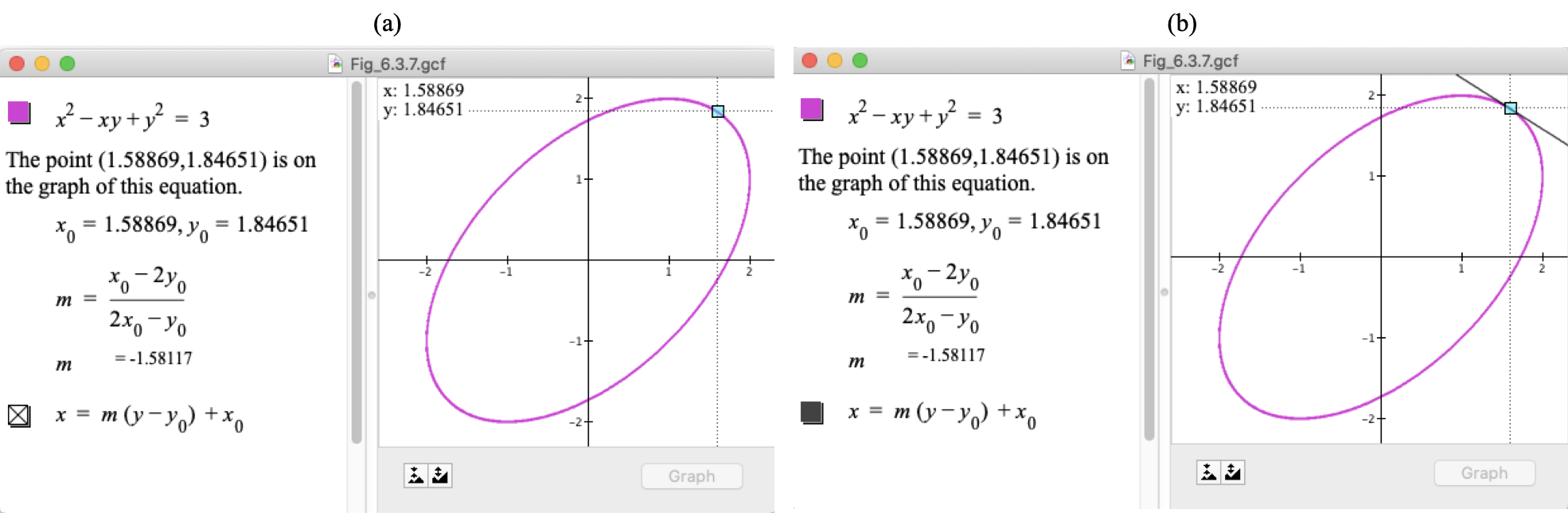
• If the rate function for g is indeed correct, then for any point $(x_0,y_0)$ on the graph of $x^2-xy+y^2=3$, the function passing through that point with a rate of change of $r_g(y_0)$ and $x=x_0$ should be tangent to the graph of $x^2-xy+y^2=3$ at $(x_0,y_0)$.
• Figure 6.3.7 demonstrates the accuracy of our test. The first pane of Figure 6.3.7 shows that the point (1.58869,1.84651) is on the graph of $x^2-xy+y^2=3$.
• The second pane of Figure 6.3.7 shows that with $x_0=1.58869$, $y_0=1.84651$, and m (our hypothesized rate of change of x with respect to y when $x=x_0$ and $y=y_0$), calculated according to Equation 6.3.10, GC’s graph of $x=m(y-y_0)+x_0)$ is indeed tangent to the graph of $x^2-xy+y^2=3$ at (1.58869,1.84651).

Figure 6.3.7. Testing Equation 6.3.10's derivation of $r_g(y)$.

The method exemplified in Equation 6.3.10, deriving the rate of change function for a function defined implicitly, is often called implicit differentiation. It is important to realize that implicit differentiation (deriving the rate of change function for a function defined implicitly) is a method. It is not a rule.

An Application of Implicitly Derived Rate Functions: Rational exponents

As an immediate application of the method of implicitly derived rate functions we will address the issue that, to this point, the power rule applies only to functions that are to an integer power.

Suppose that $y=x^\frac{p}{q}$, where p and q are integers and $q \neq 0$. If $y=x^\frac{p}{q}$, then it is also true that $y^p=(x^\frac{p}{q})^q$, or $y^q=x^p$. Using the method of implicitly defined rate functions and using the laws of exponents, we have

$$\color{red}{\text{(Eq. 6.3.11)}}\qquad \begin{align} y&=x^{p/q},\, p\text{ and }q \text{ integers, }q\neq 0\\[1ex] y^q&=x^p\\[1ex] \frac{d}{dx}y^q&=\frac{d}{dx}x^p\\[1ex] qy^{q-1}\frac{dy}{dx}&=px^{p-1}\frac{dx}{dx}\\[1ex] \frac{dy}{dx}&=\frac{px^{p-1}}{qy^{q-1}}\\[1ex] &=\left(\frac{p}{q}\right)\frac{x^{p-1}}{y^{q-1}}\\[1ex] &=\left(\frac{p}{q}\right)x^{p-1}y^{1-q} &\color{red}{\text{Note: }\frac{1}{y^{q-1}}=y^{-(q-1)}=y^{1-q}}\\[1ex] &=\left(\frac{p}{q}\right)x^{p-1}\left(x^{p/q}\right)^{1-q} &\color{red}{\text{Because $y=x^{p/q}$}}\\[1ex] &=\left(\frac{p}{q}\right)x^{p-1}x^{(p/q)(1-q)}&\color{red}{\text{Because $\left(a^b\right)^c=a^{bc}$}}\\[1ex] &=\left(\frac{p}{q}\right)x^{p-1}x^{p/q-p}\\[1ex] &=\left(\frac{p}{q}\right)x^{p-1+p/q-p}\\[1ex] &=\left(\frac{p}{q}\right)x^{p/q-1} \end{align}$$

Therefore, $$\frac{dy}{dx}=(\dfrac{p}{q})x^{p/q-1} \text{ when } y=x^{p/q} \text{ and } x^{p/q} \text{ is defined.}$$

We could also write this as $$\dfrac{d}{dx}x^{p/q}=\dfrac{p}{q}x^{\frac{p}{q}-1},$$

or as$$r_f(x)=x^{p/q-1} \text{ when } f(x)=x^{p/q}.$$

All of these statements assume that p and q are integers, $q\neq0$.

In other words, the power rule works for rational exponents as well as integers. Indeed, the power rule works for all real numbers, but the argument for the power rule working for all real numbers demands an understanding of real numbers that is beyond the scope of an introductory calculus course.

Another Application of Implicitly Derived Rate Functions: Inverse Trigonometric Functions

In this development of rate of change functions for inverse trigonometric functions, we will denote inverse sine of x as "asin(x)", which is short for "arcsine of x", instead of the often-used notation "$\sin^{-1}(x)$".

This is for two reasons:

(1) students often confuse the negative exponent to mean $\dfrac{1}{\sin(x)}$, and

(2) GC uses the notation asin(x) to mean the arc sine function--the arc length (angle measure) which produces the value $\sin(x)$.

We will similarly use "acos(x)" in place of "$\cos^{-1}(x)$" and "atan(x)" in place of "$\tan^{-1}(x)"$.

We will use several facts and relationships in the derivation of the rate of change function for asin(x), which we will denote in differential notation as $\frac{d}{dx}\asin(x)$. These are:

• $y=\asin(x)$ implies that $\sin(y)=x$, $-1 \le x \le 1$, $\dfrac{-\pi}{2} \le y \le \dfrac{\pi}{2}$. Take note that y is an arc length (in radians) and x is the value sin(y).
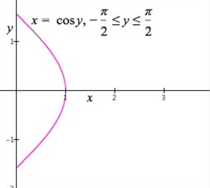
• $(\sin(y))^2+(\cos(y))^2=1$, and therefore $\cos(y)= \pm  \sqrt{1-(\sin(y))^2}$
• GC’s graph of $x=\cos(y)$ shows us that $\cos(y) \ge 0$ when $\dfrac{-\pi}{2} \le y \le \dfrac{\pi}{2}$. So, $\cos(y)= \sqrt{1-(\sin(y))^2}$ because, as the first bullet states, the value of y is indeed between $\dfrac{-\pi}{2}$ and $\dfrac{\pi}{2}$.

The deriviation of $\dfrac{d}{dx}\asin(x)$ is given in Equation 6.3.12. We derive the rate of change function for $\asin(x)$ implicitly by deriving the rate of change function for sin(y), where $y=\asin(x)$.

$$\color{red}{\text{(Eq. 6.3.12)}}\qquad \begin{align} y&=\asin(x),\, -1\lt x \lt 1\\[1ex]\sin(y)&=x&\text{Def. of inverse}\\[1ex] \frac{d}{dx}\sin(y) &=\frac{d}{dx}x\\[1ex] \cos(y)\frac{dy}{dx} &=1 & \text{Chain rule}\\[1ex] \frac{d}{dx}y&=\frac{1}{\cos(y)}&\cos(y)\ge 0\text{ since }-\pi/2\le y \le \pi/2\\[1ex] &=\frac{1}{\sqrt{1-\left(\sin(y)\right)^2}}&\cos^2(y)+\sin^2(y)=1\\[1ex] &=\frac{1}{{\sqrt{1-x^2}}}&x=\sin(y)\\[1ex] \text{Therefore, }\frac{d}{dx}\asin(x)&=\frac{1}{\sqrt{1-x^2}},\,-1\lt x\lt 1 \end{align}$$

Or, in rate notation, $r_f(x)=\dfrac{1}{\sqrt{1-x^2}}$ when $f(x)=\asin(x), -1<x<1$.

It is left as exercises for you to use the same method as above to derive the rate of change functions for acos(x) and atan(x).

Exercise Set 6.3.9

1. Confirm Equation 6.3.10 by clicking on the graph of $x^2-xy+y^2=3$ at several points, recording their coordinates, and modifying the GC statements in Figure 6.3.7 accordingly.

2. In Equation 6.3.10 we assumed that x is a function of y. Repeat Equation 6.3.10 with the assumption that y is a function of x, then test your derivation in the same way as in Figure 6.3.7.

3. Repeat the derivation in Equation 6.3.9 twice, first using rate notation then using prime notation.

4. Assume that $y=g(x)$ in each of a-c. Find the exact rate of change function $r_g$ for each. Use any notational system that is convenient. Check your derivation by graphing it along with the graph of g’s approximate rate function.

1. $y=x^2 y^3 + y^4 x$
2. $x=x^2-y^2,x>0$
3. $\sin^2(x)+\cos^2(y)=\cos(x+y)$

5. Find the exact rate of change function, $r_f(x)$, for each function $f(x)$ shown below. Check your derivation by graphing it along with the graph of f’s approximate rate function.

1. $f(x)=\tan(\sqrt{x})$
2. $f(x)=\cos^2 (5x^4)$
3. $f(x)=x \dfrac{200-3x}{\pi}$
4. $f(x)=(\sqrt[5]{x^4})(x-2x^4)$
5. $f(x)=\dfrac{5x^3-6x+9}{2x-7}$
6. $f(x)=\dfrac{3 \sqrt[5]{x^2}}{2x-8}+3(x-8)^{-4}-\sec^2(x)$

6. For each of 5c and 5d, use your work to find $\displaystyle{\int_a^x r_f(t)dt}$ in closed form. What do you notice?

7. A 10-foot ladder leans against a wall.  A mischievous monkey kicks the ladder so that its bottom slides along the floor (see animation below). The bottom of the ladder is initially 0 feet from the wall.  The bottom moves away from the wall at a rate of 1.3 feet per second.




1. Define a function h whose values give the ladder’s height on the wall at each moment in time that the ladder falls.
2. When does the ladder hit the floor?
3. Derive the exact rate of change function, $r_h$, whose values give the rate at which the height of the ladder is varying at each moment in time. Check your derived function by graphing it along with the graph of h’s approximate rate function.
4. Graph $y=r_h(x)$ over an appropriate interval, where x is the number of seconds that the ladder has fallen. Does the ladder’s top ever fall faster than would a ball were it released from a height of 10 feet, falling under the influence of gravity?

8. A man having a height of 1.75 meters stood under a street light, then walked away it at a rate of 1.7 meters per second.  The streetlight is 6 meters above the street. The streetlight casts a shadow in front of him.

1. Define a function s that relates the length of the man’s shadow to the distance he has walked from the streetlight at any particular moment in time since leaving the streetlight.
2. How long is the man’s shadow after 5 seconds? 
3. Define a function $r_s$, in closed form, whose values give the rate at which the man’s shadow lengthens with respect to the number of seconds since he left the streetlight. Check your derivation by graphing it along with the graph of s’s approximate rate function.
4. Define an integral based on $r_s$ that gives the length of the man’s shadow x seconds after leaving the streetlight. What is the closed form representation of that integral?

9. Use the method of deriving a rate of change function implicitly to show that $r_f(x)=\dfrac{1}{1+x^2}$ when $f(x)=\atan(x)$. Use these facts:

   • $y=\atan(x)$ means that $\tan(y)=x$;
   • $(\sec(y))^2=1+(\tan(y))^2$.

   Restrict the value of x appropriately in $r_f(x)$.

   Check your derivation by graphing it along with the graph of $y=\dfrac{f(x+0.001)-f(x)}{0.001}$.

10. Use the method of deriving a rate of change function implicitly to show that $r_f(x)=-\dfrac{1}{1-x^2}$ when $f(x)=\acos(x)$. Use these facts:

    • $y=\acos(x)$ means that $\cos(y)=x$;
    • $\acos(x)+\asin(x)=\pi/2$.

    Restrict the value of x appropriately in $r_f(x)$.

    Check your derivation by graphing it along with the graph of $y=\dfrac{f(x+0.001)-f(x)}{0.001}$.

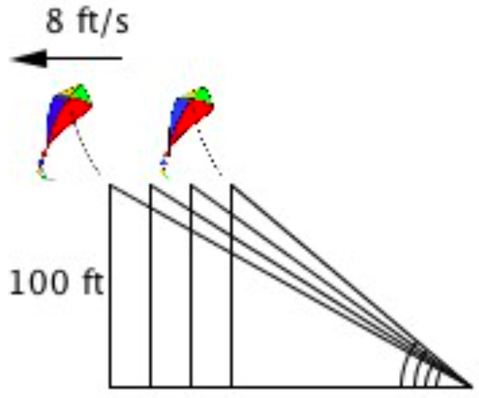
11. The diagram below shows a kite 100 ft above the ground moves horizontally away from you at a rate of 8 feet per second. The kite’s height does not vary, but the angle made by the ground and the kite string varies as the kite moves away from you.

1. Define a function that gives the rate of change of the string’s angle with the ground at every moment in time. Check your definition by graphing it along with the graph of your function’s approximate rate function.
2. At what rate is the angle between the string and the ground varying when 150 feet of the string has been let out? 



12. The animation below shows the hands of a large clock rotating rapidly. The hour hand is 1.5 meters long; the minute hand is 4 meters long. Define a function whose values give the rate at which the distance between the tips of the hour and minute hands varies with respect to the measure of the angle between them.

6.3.10 Derived Rate of Change Functions for Exponential and Log Functions

In this section we will first review the ideas of exponential and logarithmic functions and then derive rate of change functions for them in closed form.

Exponential Functions

Paal Payasam is an Indian dish made of milk and rice. The  Legend of Paal Payasam illustrates the immensity of exponential growth.

The legend is that Lord Krishna played a game of chess against King Rhada for this bet: If Krishna won, the King must give him 1 grain of rice on the board’s first square, 2 grains on the second, 4 grains on the third, and $2^{n-1}$ grains on the $n^{th}$ square, up to $n=64$.

Krishna won the game, and King Rhada quickly understood the foolishness of his bet. He foresaw having to put 4.29 billion grains of rice on the $33^{rd}$ square and 9.22 billion billion grains on the $64^{th}$ square--a number of grains of rice that would cover all of India.

The expressions $x^b$ and $b^x$ have similar forms, but they have entirely different meanings and, as illustrated by the Legend of Pall Paysam, entirely different behaviors.

When we say $y=x^b$, we are saying that for any value of x, the value of y contains x as a factor b times. If $b=2$, then y contains 2 factors of x, or $y=x \cdot x$. The value of x varies, but the number of factors does not vary.

It would be convenient if exponential functions obeyed the power rule. However, they do not.

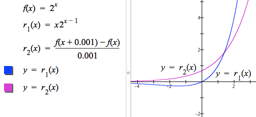
Figure 6.3.8 shows the power rule applied to $f(x)=2^x$ (see GC’s graph of $r_1$) compared to f’s approximate rate of change function (see GC’s graph of $r_2$).

We trust the approximate rate function with $h=0.001$ to be reasonably close to the exact rate of change function for f.

GC’s graph of $r_1$, which uses the power rule on f, is not even close to GC’s graph of $r_2$, f’s approximate rate function. The power rule does not apply to exponential functions.

 
Figure 6.3.8. The power rule applied to an exponential function does not match the exponential function's approximate rate of change function.

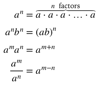
To understand the derivation of the general form of an exponential function’s rate of change function you must recall properties of exponents. As a reminder:

Two special cases are when $a=0$ or $n = 0$ in $a^n$.

• First, when $a\neq 0$ we define $a^0=1$ to be consistent with the fact $\dfrac{a^m}{a^n}=a^{m-n}$.
  When $n=m$ and $a\neq0$, $\dfrac{a^m}{a^n}=a^{m-n}=a^0=1$. This is why we define $a^0$ to be 1.
• We define $0^0$ to be 1 so the graph of $y=x^0$ is continuous at $x=0$. All values of $x^0$ are then 1.

The derivation of the rate of change function for $f(x)=b^x$ is given in Equation 6.3.13.

The derivation starts by defining the approximate rate function r, and deriving the statement $r(x)=b^x(\frac{b^h-1}{h})$.

That is, the rate of change function for $f(x)=b^x$ is a product of $b^x$ and the expression $\dfrac{b^h-1}{h}$. We cannot let $h=0$ because $\frac{b^0-1}{0}=\frac{0}{0}$, which is undefined.

The question we must answer, then, is whether $\frac{b^h-1}{h}$ represents a number when $h$ is indistinguishable from zero but not equal to zero.

$$\color{red}{\text{(Eq. 6.3.13)}}\qquad \begin{align} f(x)&=b^x,\,b\gt 0\\[2ex] r(x)&=\frac{f(x+h)-f(x)}{h},\, h\neq 0\\[1ex] &=\frac{b^{x+h}-b^x}{h}\\[1ex] &=\frac{b^xb^h-b^x}{h}\\[1ex] &=\frac{b^x\left(b^h-1\right)}{h}\\[1ex] &=b^x\left(\frac{b^h-1}{h}\right) \end{align}$$

Equation 6.3.13 ends with $b^x$ multiplied by $(b^h-1)/h$. At this moment we don't know what to make of $(b^h-1)/h$.

Figure 6.3.9 investigates the behavior of $\dfrac{b^x-1}{x}$ around $x=0$ for various values of b from 0 to 500.

When you play the animation in Figure 6.3.9 you should see:

• For $b=0$, $\dfrac{b^x-1}{x}$ has $x=0$ as a vertical asymptote.

• For values of $b>0$, it appears that $\dfrac{b^x-1}{x}$ is always essentially equal to some number for $x \doteq 0$, although it is a different number for each value of b.

The main point of Figure 6.3.9 is that $(b^h-1)/h$ is always equal to some number when $h \neq 0$ and $b>0$. But the value of $(b^h-1)/h$ depends on the value of b.

For the meantime, we’ll represent $(b^h-1)/h$ as $c_b$ to remind us that $(b^h-1)/h$ is a number for $h \neq 0$. We use "sub b" in $c_b$ to remind us that this number depends on the value of b.

When $f(x)=b^x, b>0$, we have that $r_f(x)=c_b b^x$, where the value of $c_b$ depends on the value of b.

For some value of b, $c_b$ is essentially equal to 1 when $h \doteq 0$.

In honor of Leonard Euler, we give the special symbol e to the value of b that makes $\dfrac {b^h-1}{h}\doteq 1$ when $h\doteq 0$. Therefore $c_e=1$ by definition of e.

The importance of the value of b that makes $c_b=1$ is that the rate function for this exponential function is $r_f(x)=f(x)$ when $f(x)=e^x$.

In differential notation, $\dfrac{d}{dx}e^x=e^x$.

The value of e is irrational. Its value is approximately 2.71828 (to 5 decimal places). The history of attempts to approximate the value of e is fascinating. See Eli Maor’s excellent account of this history.

Logarithmic Functions

A logarithmic function is the inverse of an exponential function, and thus its definition depends on the base of the exponential function for which it is inverse. In other words,

For $b>0$, $\log_b(x)=y$ such that $b^y=x$

So $\log_3(81)=y$ such that $3^y=81$. Therefore $\log_3(81)=4$, because $3^4=81$. Also, $\log_{\frac{1}{3}}(81)=-4$ because $\left(\dfrac{1}{3}\right)^{-4}=81$.

We can use the inverse relationship between $\log_b$ and $b^x$ and the method of implicitly derived rate functions to find the derived rate of change function for f defined as $f(x)=\log_b(x), b>0$.

Equation 6.3.14 starts by stating the inverse relationship between exponential and logarithmic functions and then uses the method of implictly derived rate functions and the chain rule to end with the derived rate function for $y=\log_b(x)$.

$$\color{red}{\text{(Eq. 6.3.14)}}\qquad \begin{align} \log_b(x)&=y\text{ means that $b^y=x$} & \text{Def. of Inverse Function}\\[1ex] \frac{d}{dx}\log_b(x)&=\frac{d}{dx}y\text{ means that }\frac{d}{dx}b^y=\frac{d}{dx}x\\[1ex] \text{Derivation:}\\[1ex] \frac{d}{dx}b^y&=\frac{d}{dx}x\\[1ex] c_b \frac{d}{dx}y&=1 & \text{Chain rule}\\[1ex] \frac{d}{dx}y&=\frac{1}{c_b b^y}\\[1ex] \frac{d}{dx}y&=\frac{1}{c_b x} & \text{Substitute $x$ for }b^y \end{align}$$

In the case where $b=e$, $c_e=1$, so we have

$$\frac{d}{dx}\log_e(x)=\frac{1}{c_e x}\text{, or}$$ $$\frac{d}{dx}\log_e(x)=\frac{1}{x}.$$

Reflection 6.3.4. Why do we include the restrictions $b>0$ and $x>0$ in the definition of a logarithm function? Hint: Suppose that we allowed $b≤0$ or $b=1$? What would go wrong? What about values of $x≤0$?

Because $e^x$ has the special property that $\dfrac{d}{dx} e^x=e^x$, and because $\log_e(x)$ has the special property that $\dfrac{d}{dx}\log_e(x)=\dfrac{1}{x}$, e is called the natural base of the exponential and log functions.

The natural log is denoted "ln" (from Latin, logarithmus naturalis).

In the future we will write $\log_e(x)$ as $\ln(x)$, and we will call $\ln(x)$ the natural log of x.

Equation 6.3.15 gives us the opportunity to determine the value of this ubiquitous constant $c_b=\dfrac{b^h-1}{h}$ for $h \doteq 0$.

In determining $c_b$ we  will use the simplicity of the derived rate function for $f(x)=e^x$ together with the fact that $b^{\log_b(x)}=x$ for any value of $b>0$ and for any value of $x>0$.

Now we use the fact that $b^x=e^{\ln b^x}$ to determine the value of $c_b$ in $\dfrac{d}{dx}b^x=c_b b^x$.

$$\color{red}{\text{(Eq. 6.3.15)}}\qquad \begin{align} b^x&=e^{\ln b^x}\\[1ex] &=e^{x\ln b}\\[1ex] \frac{d}{dx}b^x&=\frac{d}{dx}e^{x\ln b}\\[1ex] &=e^{x\ln b}\frac{d}{dx}x\ln b & \text{Chain rule}\\[1ex] &=e^{x\ln b}\ln b\\[1ex] &=(\ln b)b^x & \text{Substitute }b^x\text{ for }e^{x \ln b}\\[2ex] \text{Therefore, }c_b&=\ln b\\[1ex] \frac{b^h-1}{h}&= \ln b\text{ for }h\doteq 0 \end{align}$$

In summary, and in differential notation:

The case of $\dfrac{d}{dx}\ln(x)=\dfrac{1}{x}$ deserves more consideration.

$\ln(x)$ is defined only when $x>0$. However, $\dfrac{1}{x}$ is defined when $x>0$ and when $x<0$. The question therefore becomes,

Figure 6.3.10 addresses this question. It shows that $\int_a^x \frac{1}{t}dt$ is defined for $a<0$ and $x<0$ as well as for $a>0$ and $x>0$.

Figure 6.3.10 also demonstrates that the graphs of $\displaystyle{\int_a^x \frac{1}{t}dt}$ coincides with the graph of $y=\ln(-x)-\ln(-a)$ when a and x are both negative.

We can therefore say that $\int_a^x \frac{1}{t}dt = \ln(|x|)-\ln(|a|)$ when a and x are both negative or both positive.

We cannot integrate $\frac{1}{t}$ over an interval that includes 0 because $\frac{1}{t}$ is undefined for $t=0$, and, as we will see later, $\int_0^c \frac{1}{t}dt$ is infinite for any value of c.

Exercise Set 6.3.10

1. Make an updated library of ROC/Integral pairs.

2. Show that $\log_3(x)$ can be expressed as $\dfrac{\ln(x)}{\ln(3)}$.

3. Show that $\log_b(x)$ can be expressed as $\dfrac{\ln(x)}{\ln(b)}$. Use this fact to graph $y=\log_7(x)$.

4. Find the exact rate of change function for each of (a) and (b), below. Check your derivations by graphing them along with the graph of $y=\dfrac{m(x+0.001)-m(x)}{0.001}$.


1. $m(t)=7\ln(8-t)+t^2-\dfrac{1}{2}$


2. $m(r)=\log_{10}(2+\cos(r))$


5. A logistic population model often is used in the biological and ecological sciences to model the growth of animal populations.  This model takes into account the population’s initial size $P_0$, its growth rate r per time unit, the environment’s carrying capacity K (the maximum number of animals the environment can sustain), and the value of m (the moment when the expected population will be half its carrying capacity).  Values of the function P, defined as
   
   
   $$P(t)=\frac{P_0 K}{P_0 + (K-P_0)e^{-r(t-m)}}$$
   
   give the population size after t months have elapsed.  $P_0$ is the initial population size, K is the carrying capacity, and r is the exponential growth rate for the population. Let $m = 50$.


1. Identify parameters and variables in the function definition.


2. Create a slider in GC that will allow you to analyze carrying capacities ranging from 2000 to 4000.


3. Create another slider in GC that will allow you to analyze initial populations ranging from 100 to 1000.


4. Create a third slider in GC that allows you to analyze growth rates from 0.002 to 0.05.


5. Explain how each parameter affects population growth.


6. We would like to find an exact rate of change function $r_P$ so that we can analyze how the rate of change of the population with respect to the number of days elapsed affects the population’s growth rate.  Derive $r_P$, then define it in GC. Check your derivation with the approximate rate function for P.


7. Given an initial population of 100 individuals, a carrying capacity of 2500, and $r=.35$, use GC to evaluate the population after 42 months from time $t=0$.


8. For this same population, compute $r_P(42)$ and explain what this value represents about the population.


9. How might a game warden make use of the graph of P’s rate of change function?


6. Brenan monitors the rate at which water is moving in a stream along the Colorado River during a rainstorm.  He places his measurement instrument in the river; it records how fast the river is flowing in $\mathrm{\frac{m}{sec}}$.
   
   From his map of the river bed, Brenan estimates the cross-sectional area of the river at the point where he takes his measurements. He then enters this cross sectional area into his instrument’s radio controller. With the river’s cross-sectional area and the rivers speed,  the instrument can compute the flow rate, in cubic meters per second.  The measurement tool also records how many hours have elapsed since being placed in the river.  For more information if you are interested on how these measurements are taken by hydraulic scientists go here.
   
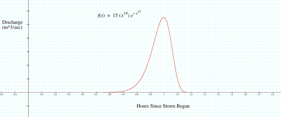
   Brenan returned after a rainstorm to pick up his equipment.  He went back to the lab where he created a mathematical model of the flow rate—a function whose values give the water’s flow rate at each moment in time during the recording.  Here is Brenan’s model: $f(x)=15(x^{14})e^{-x^{15}}$, where values of f are a flow rate x hours after recording began.


1. Approximate the time the river’s flow rate changes from increasing to decreasing.


2. Approximate the time the river’s flow changes from increasing to decreasing.


3. At approximately what moment in time does the river’s flow stop accelerating and start decelerating?  Does the flow begin to accelerate again at any point?  If so, approximately when does this acceleration occur?




4. Brenan’s boss is worried that the local dam has gained too much water in its reservoir. He needs to know how much water passed that point in the river during the recorded time.  How much water flowed past the instrument during this period of time?

6.3.11 Derived Rate of Change Functions for Functions h in the form $h(x)=f(x)^{g(x)}$

In this section we will derive rate of change functions for functions of the form $h(x)=f(x)^{g(x)}$. Functions in this form are not power functions, since the exponent is not constant, and they are not exponential functions, since the base is not constant.

Briggs, Cochran, Gillet, and Schultz (2011) propose to call functions of the form $h(x)=f(x)^{g(x)}$ tower functions. We will adopt Briggs et al.’s proposal.

Suppose that h is defined as $h(x)=g(x)^{f(x)}$ and that f and g have rate of change functions $r_f$ and $r_g$. We do not have a method for deriving h’s rate of change function.

Just as in much of mathematics, our question is not so much about how to do something, but how to represent what we want to act upon so that we can use the methods that we have. We ask, "How can we represent the function $h(x)=g(x)^{f(x)}$ in an equivalent form so that we can use existing methods?"

We can rewrite the definition of h using the identities $g(x)=e^{\ln(g(x))}$ and $\ln(x^y)=y\ln x$ to put the definition of h in a form where we do have methods to derive its rate of change function.

Before we do this, however, we must point out that $g(x)$ and $e^{\ln(g(x))}$ are not always equivalent. Because $\ln(u)$ is defined only for values of $u>0$, the expression $e^{\ln(g(x))}$ is defined only for values of x such that $g(x)>0$.

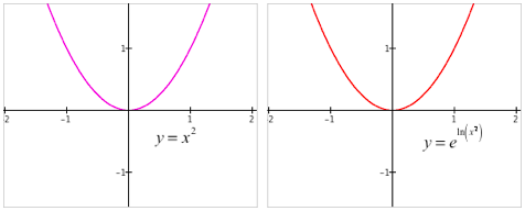
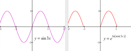
Figure 6.3.11 illustrates the constraint that $g(x)$ must be greater than 0. The first pane in Figure 6.3.11 shows GC’s graphs of $y=x^2$ and $y=e^{\ln(x^2)}$ being identical. The second pane shows that GC’s graphs of $y=\sin(3x)$ and $y=e^{\ln(\sin(3x))}$ are identical only for values of x such that $\sin(3x)>0$.

(a)

(b)

    
Figure 6.3.11. Look between each pair of panes. The statement $y=e^{\ln(f(x))}$ produces same graph as $y=f(x)$, but only for values of x such that $f(x)>0$.

Suppose $g(x)\gt 0$ for all values of x, and f and g have rate of change functions $r_f$ and $g_f$. We will use two identities in the derivation of $r_h$ where $h(x)=g(x)^{f(x)}$. These properties are:

We also will use the chain rule several times, and the derived functions for products and logs. The derivation of $r_h$ where $h(x)=g(x)^{f(x)}$, $g(x)>0$ is given in Equation 6.3.17.

$$\color{red}{\text{(Eq. 6.3.17)}}\qquad \begin{align} h(x)&=g(x)^{f(x)}\\[1ex] &=e^{f(x)\ln(g(x))},\, g(x)\gt 0\\[1ex] r_h(x) &=\frac{d}{dx}e^{f(x)\ln(g(x))}\\[1ex] &=e^{f(x)\ln(g(x))}\frac{d}{dx}\left(f(x)(\ln(g(x))\right) & \text{Chain rule}\\[1ex] \frac{d}{dx}f(x)\ln(g(x)) &=f(x)\frac{d}{dx}\ln(g(x))+\ln(g(x))\frac{d}{dx}f(x) & \text{Product rule}\\[1ex] &=f(x)\left(\frac{1}{g(x)}\right)\frac{d}{dx}g(x)+\ln(g(x))\frac{d}{dx}f(x) & \text{ln and chain rules}\\[1ex] &=\frac{f(x)}{g(x)}r_g(x)+\ln\left(g(x)\right)r_f(x)\\[1ex] r_h(x) &=g(x)^{f(x)}\left(\frac{f(x)}{g(x)}r_g(x)+\ln\left(g(x)\right)r_f(x)\right),\, g(x)\gt 0 \end{align}$$

Reflection 6.3.7. What is $r_f(x)$ when $f(x)=x^x$? Over what domain is $r_f$ defined?

Reflection 6.3.8. Examine GC’s graph of $y=x^x$. Why is it reasonable to adopt the convention that $0^0=1$ even though, logically, $0^0$ is undefined?

Exercise Set 6.3.11

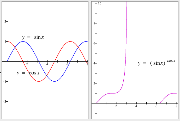
1. In the figure below, the graphs of $y=\sin(x)$ and $y=\cos(x)$, $0 \le x \le 8$ are displayed in the left graphing pane; the graph of $y=(\sin(x))^{\cos(x)}$, $0 \le x \le 8$, is shown in the right graphing pane. Why does the graph of $y=(\sin(x))^{\cos(x)}$ increase so dramatically where it does? (Think about a really small number being raised to a negative power.) Why does the graph have gaps where it does?





2. Examine GC’s graph of $f(x)=(\cos(x))^x$. (Zoom out so that you can see at least $-20<x<20$.)

1. Explain, in terms of values of $\cos(x)$ and values of x, why the graph of f behaves as it does.
   


2. Determine $r_f$, the exact rate of change function for f.  Explain the behavior of $y=r_f(x)$ in terms of the behavior of $y=f(x)$.


3. Derive the exact rate of change function $r_k$ in closed form for each function k shown below. Check your answers using this GC file. Study the behavior of $r_k$ to see that it reflects the behavior of k.


1. $k(x)=(2x)^{-3x}$


2. $k(t)=e^{\ln(5t^3-2t^2+3t-4)}$


3. $k(u)=(u^4-8)^{7u \cos(3u^2-4)}$


4. $k(t)=(t^2+4)^m$


4. Derive the exact rate of change function $r_f$ in closed form for each function f shown below. Check your answers using this GC file. Study the behavior of $r_f$ to see that it reflects the behavior of f.


1. $f(x)=10^{\log(3x-7)}$


2. $f(x)=\ln(e^{\sin(x)})$


3. $f(x)=(3x-4)^{e^x}$


4. $f(x)=\left(\dfrac{1}{(x-5)^2}\right)^{\sqrt{x-3}}$

6.3.12 Big Assumptions We Made (in progress)

6.3.13 The Mean Value Theorem (in progress)